Independent t-test using Stata

Introduction

The independent t-test, also referred to as an independent-samples t-test, independent-measures t-test or unpaired t-test, is used to determine whether the mean of a dependent variable (e.g., weight, anxiety level, salary, reaction time, etc.) is the same in two unrelated, independent groups (e.g., males vs females, employed vs unemployed, under 21 year olds vs those 21 years and older, etc.). Specifically, you use an independent t-test to determine whether the mean difference between two groups is statistically significantly different to zero.

For example, an independent t-test could be used to test whether revision time amongst college students differed based on gender (i.e., your dependent variable would be "revision time", measured in minutes or hours, and your independent variable would be "gender", which has two groups: "male" and "female"). Alternately, an independent t-test could be used to understand whether there is a difference in salary based on educational level (i.e., your dependent variable would be "salary" and your independent variable would be "educational level", which has two groups: "undergraduate degree" and "postgraduate degree").

Note: In Stata 12, you will see that the independent t-test is referred to as the "two-group mean-comparison test", whereas in Stata 13, it is referred to as the "t test (mean-comparison test)".

In this guide, we show you how to carry out an independent t-test using Stata, as well as interpret and report the results from this test. However, before we introduce you to this procedure, you need to understand the different assumptions that your data must meet in order for an independent t-test to give you a valid result. We discuss these assumptions next.

Note: If your independent variable has related groups, you will need to use a paired t-test instead. Alternatively, if you have more than two unrelated groups, you could use a one-way ANOVA. However, if you only have one group and wish to compare this to a known or hypothesized value, you could run a one-sample t-test. We also have a guide on how to run an independent t-test using Minitab.

Stata

Assumptions

There are six "assumptions" that underpin the independent t-test. If any of these six assumptions are not met, you cannot analyse your data using an independent t-test because you will not get a valid result. Since assumptions #1, #2 and #3 relate to your study design and choice of variables, they cannot be tested for using Stata. However, you should decide whether your study meets these assumptions before moving on.

• Assumption #1: Your dependent variable should be measured at the interval or ratio level (i.e., they are continuous). Examples of such dependent variables include height (measured in feet and inches), temperature (measured in ^oC), salary (measured in US dollars), revision time (measured in hours), intelligence (measured using IQ score), reaction time (measured in milliseconds), test performance (measured from 0 to 100), sales (measured in number of transactions per month), and so forth. If you are unsure whether your dependent variable is continuous (i.e., measured at the interval or ratio level), see our Types of Variable guide.
• Assumption #2: Your independent variable should consist of two categorical, independent (unrelated) groups. Examples of such independent variables include gender (2 groups: male or female), treatment type (2 groups: medication or no medication), educational level (2 groups: undergraduate or postgraduate), religious (2 groups: yes or no), and so forth.
• Assumption #3: You should have independence of observations, which means that there is no relationship between the observations in each group or between the groups themselves. For example, there must be different participants in each group with no participant being in more than one group. If you do not have independence of observations, it is likely you have "related groups", which means you will need to use a dependent t-test instead of the independent t-test.

Fortunately, you can check assumptions #4, #5 and #6 using Stata. When moving on to assumptions #4, #5 and #6, we suggest testing them in this order because it represents an order where, if a violation to the assumption is not correctable, you will no longer be able to use an independent t-test. In fact, do not be surprised if your data fails one or more of these assumptions since this is fairly typical when working with real-world data rather than textbook examples, which often only show you how to carry out an independent t-test when everything goes well. However, don’t worry because even when your data fails certain assumptions, there is often a solution to overcome this (e.g., transforming your data or using another statistical test instead). Just remember that if you do not check that your data meets these assumptions or you test for them incorrectly, the results you get when running an independent t-test might not be valid.

• Assumption #4: There should be no significant outliers. An outlier is simply a single case within your data set that does not follow the usual pattern (e.g., in a study of 100 students' IQ scores, where the mean score was 108 with only a small variation between students, one student had a score of 156, which is very unusual, and may even put her in the top 1% of IQ scores globally). The problem with outliers is that they can have a negative effect on the independent t-test, reducing the accuracy of your results. Fortunately, when using Stata to run an independent t-test on your data, you can easily detect possible outliers.
• Assumption #5: Your dependent variable should be approximately normally distributed for each category of the independent variable. Your data need only be approximately normal for running an independent t-test because it is quite "robust" to violations of normality, meaning that this assumption can be a little violated and still provide valid results. You can test for normality using the Shapiro-Wilk test of normality, which is easily tested for using Stata.
• Assumption #6: There needs to be homogeneity of variances. You can test this assumption in Stata using Levene's test for homogeneity of variances. Levene's test is very important when it comes to interpreting the results from an independent t-test guide because Stata is capable of producing different output depending on whether your data meets or fails this assumption.

In practice, checking for assumptions #4, #5 and #6 will probably take up most of your time when carrying out an independent t-test. However, it is not a difficult task, and Stata provides all the tools you need to do this.

In the section, Test Procedure in Stata, we illustrate the Stata procedure required to perform an independent t-test assuming that no assumptions have been violated. First, we set out the example we use to explain the independent t-test procedure in Stata.

Stata

Example

With a large proportion of heavy smokers struggling to quit, the government wants to find ways to help them reduce their cigarette consumption. A researcher wants to investigate whether the use of nicotine patches reduces cigarette consumption, and if so, by how much.

Therefore, the researcher recruits a random sample of 30 heavy smokers from the population, where a heavy smoker is defined as a person who smokes an average of 40 cigarettes or more per day. This sample of 30 participants was randomly split into two independent groups – a "control group" and a "treatment group" – with 15 participants in each group. Therefore, 15 participants were given the nicotine patches (the treatment group) and 15 participants were given a "placebo"; that is, a patch that did not contain any nicotine (the control group). As a result, none of the participants knew whether they were in the treatment group or the control group. Three months after the start of the experiment, the cigarette consumption of the two groups was measured in terms of the average number of cigarettes smoked per day. Therefore, the dependent variable was "cigarette consumption" (measured in terms of the number of cigarettes smoked daily at the end of the experiment), whilst the independent variable was "treatment type", where there were two independent groups (the treatment group and control group).

An independent t-test was used to determine whether there was a statistically significant difference in cigarette consumption between the two independent groups (i.e., the treatment group and control group).

Stata

Setup in Stata

In Stata, we separated the two groups for analysis by creating a grouping variable, called TreatmentType, and gave the control group who received the placebo a value of "1 -- Placebo" and the treatment group who received the nicotine patches a value of "2 -- Nicotine patch", as shown below.

Published with written permission from StataCorp LP.

The scores for the dependent variable, CigaretteConsumption, were then entered into the Data Editor (Edit) spreadsheet in the column to the right of the independent variable, TreatmentType, as shown below:

Published with written permission from StataCorp LP.

Stata

Test Procedure in Stata

In this section, we show you how to analyse your data using an independent t-test in Stata when the six assumptions in the previous section, Assumptions, have not been violated. You can carry out an independent t-test using code or Stata's graphical user interface (GUI). After you have carried out your analysis, we show you how to interpret your results. First, choose whether you want to use code or Stata's graphical user interface (GUI).

Code

The code to run an independent t-test on your data takes the form:

ttest DependentVariable, by(IndependentVariable)

This code is entered into the box below:

Published with written permission from StataCorp LP.

Using our example where the dependent variable is CigaretteConsumption and the independent variable is TreatmentType, the required code would be:

ttest CigaretteConsumption, by(TreatmentType)

Note 1: You need to be precise when entering the code into the box. The code is "case sensitive". For example, if you entered "cigaretteConsumption" where the first "c" is lowercase rather than uppercase (i.e., a big "C"), which it should be, you will get an error message like the following:

Note 2: If you're still getting the error message in Note 1: above, it is worth checking the name you gave your dependent and independent variables in the Data Editor when you set up your file (i.e., see the Data Editor screen above). In the box on the right-hand side of the Data Editor screen, it is the way that you spelt your variables in the section, not the section that you need to enter into the code (see below for our independent variable). This may seem obvious, but it is an error that is sometimes made, resulting in the error in Note 1 above.

Therefore, enter the code, ttest CigaretteConsumption, by(TreatmentType), and press the "Return/Enter" button on your keyboard.

Published with written permission from StataCorp LP.

You can see the Stata output that will be produced here.

Graphical User Interface (GUI)

The three steps required to run an independent t-test in Stata 12 – known as a two-group mean-comparison test in Stata 12 – are shown below. The same procedure requires four steps in Stata 13 and this is shown further down:

Stata

Version 12

1. In Stata 12, click Statistics > Summaries, tables, and tests > Classical tests of hypotheses > Two-group mean-comparison test on the top menu, as shown below;
   

   Published with written permission from StataCorp LP.

   
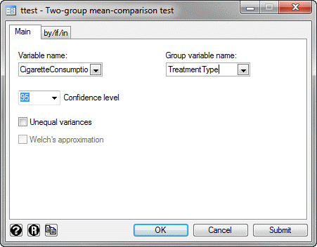
   You will be presented with the ttest - Two-group mean-comparison test dialogue box:
   
   

   Published with written permission from StataCorp LP.

2. Select the dependent variable, CigaretteConsumption, from within the Variable name: drop-down box, and the independent variable, TreatmentType, from the Group variable name: drop-down box, as shown below:
   

   Published with written permission from StataCorp LP.

3. Click on the button. This will generate the output.

Stata

Version 13

1. In Stata 13, click Statistics > Summaries, tables, and tests > Classical tests of hypotheses > t test (mean-comparison test) on the top menu, as shown below.
   

   Published with written permission from StataCorp LP.

   
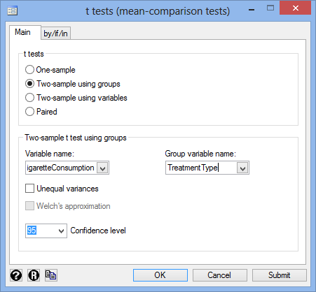
   You will be presented with the t tests (mean-comparison tests) dialogue box:
   
   

   Published with written permission from StataCorp LP.

2. Select the Two-sample using groups option in the –t-tests– area, as shown below:
   

   Published with written permission from StataCorp LP.

3. Select the dependent variable, CigaretteConsumption, from within the Variable name: drop-down box, and the independent variable, TreatmentType, from the Group variable name: drop-down box. You will end up with a screen similar to the one below:
   

   Published with written permission from StataCorp LP.

4. Click on the button. The output that Stata produces is shown below.

Stata

Output of the independent t-test in Stata

If your data passed assumption #4 (i.e., there were no significant outliers), assumption #5 (i.e., your dependent variable was approximately normally distributed for each category of the independent variable) and assumption #6 (i.e., there was homogeneity of variances), which we explained earlier in the Assumptions section, you will only need to interpret the following Stata output for the independent t-test:

Published with written permission from StataCorp LP.

This output provides useful descriptive statistics for the two groups that you compared, including the mean and standard deviation, as well as the actual results from the independent t-test. We can see that the group means are significantly different as the p-value in the Pr(|T| > |t|) row (under Ha: diff != 0) is less than 0.05 (i.e., based on a 2-tailed significance level). Looking at the Mean column, you can see that those people who used the nicotine patches had lower cigarette consumption at the end of the experiment compared to those who received the placebo.

Note: We present the output from the independent t-test above. However, since you should have tested your data for the assumptions we explained earlier in the Assumptions section, you will also need to interpret the Stata output that was produced when you tested for them. This includes: (a) the boxplots you used to check if there were any significant outliers; (b) the output Stata produces for your Shapiro-Wilk test of normality to determine normality; and (c) the output Stata produces for Levene's test for homogeneity of variances. Also, remember that if your data failed any of these assumptions, the output that you get from the independent t-test procedure (i.e., the output we discuss above) will no longer be relevant, and you will need to interpret the Stata output that is produced when they fail (i.e., this includes different results).

Stata

Reporting the output of the independent t-test

When you report the output of your independent t-test, it is good practice to include: (a) an introduction to the analysis you carried out; (b) information about your sample, including how many participants were in each group of your two groups (N.B., this is particularly useful if the group sizes were unequal or if there were missing values); (c) the mean and standard deviation for your two independent groups; and (d) the observed t-value (t), degrees of freedom (degrees of freedom), and significance level, or more specifically, the 2-tailed p-value (Pr(|T| > |t|)). Based on the results above, we could report the results of this study as follows:

In addition to the reporting the results as above, a diagram can be used to visually present your results. For example, you could do this using a bar chart with error bars (e.g., where the errors bars could be the standard deviation, standard error or 95% confidence intervals). This can make it easier for others to understand your results. Furthermore, you are increasingly expected to report "effect sizes" in addition to your independent t-test results. Effect sizes are important because whilst the independent t-test tells you whether the difference between group means is "real" (i.e., different in the population), it does not tell you the "size" of the difference. Whilst Stata will not produce these effect sizes for you using this procedure, there is a procedure in Stata to do so.