Independent t-test using Minitab

Introduction

The independent t-test (also known as an independent-samples t-test, independent-measures t-test or unpaired t-test) determines whether there is a statistically significant difference in the mean of a dependent variable between two unrelated, independent groups.

For example, you could use an independent t-test to determine whether there is a difference in stress levels amongst the long-term unemployed between households with children and households without children (i.e., the dependent variable would be "stress levels", and the independent variable would be "family status", which has two groups: "households with children" and "households without children"). Alternately, you could use an independent t-test to determine whether there is a difference in exam performance between males and females (i.e., the dependent variable would be "exam performance" and the independent variable would be "gender", which has two groups: "males" and "females"). If you have more than two independent groups, you need to run a one-way ANOVA.

Note: If you only have one sample, but wish to compare this to a known or hypothesized population mean, you will need to run a one-sample t-test. Alternately, if your independent variable is continuous, you might wish to run a linear regression analysis. If you have two independent variables rather than one, you might want to run a two-way ANOVA instead.

In this guide, we show you how to carry out an independent t-test using Minitab, as well as interpret and report the results from this test. However, before we introduce you to this procedure, you need to understand the different assumptions that your data must meet in order for an independent t-test to give you a valid result. We discuss these assumptions next.

Minitab

Assumptions

The independent t-test has six "assumptions". You cannot test the first three of these assumptions with Minitab because they relate to your study design and choice of variables. However, you should check whether your study meets these three assumptions before moving on. If these assumptions are not met, there is likely to be a different statistical test that you can use instead. Assumptions #1, #2 and #3 are explained below:

• Assumption #1: Your dependent variable should be measured at a continuous level (i.e., they are interval or ratio variables). Examples of continuous variables include height (measured in feet and inches), temperature (measured in ^oC), salary (measured in US dollars), revision time (measured in hours), intelligence (measured using IQ score), firm size (measured in terms of the number of employees), age (measured in years), reaction time (measured in milliseconds), grip strength (measured in kg), power output (measured in watts), test performance (measured from 0 to 100), sales (measured in number of transactions per month), academic achievement (measured in terms of GMAT score), and so forth. If you are unsure whether your dependent variable is continuous (i.e., measured at the interval or ratio level), see our Types of Variable guide.
• Assumption #2: Your independent variable should consist of two categorical, independent (unrelated) groups. Examples of such independent variables include gender (two groups: male or female), treatment type (two groups: medication or no medication), educational level (two groups: undergraduate or postgraduate), health insurance (two groups: yes or no), intensity of religious practice (two groups: practicing or non-practicing), personality type (two groups: introversion or extroversion), and so forth.
• Assumption #3: You should have independence of observations, which means that there is no relationship between the observations in each group or between the groups themselves. Therefore, there must be different participants in each group with no participant being in more than one group. For example, if you wanted to determine whether there was a statistically significant difference in mean anxiety level between undergraduates and postgraduates (i.e., your two independent groups), a participant cannot be both an undergraduate and a postgraduate. The participant can only be an undergraduate or a postgraduate. The participant cannot be in both groups. If you do not have independence of observations, it is likely you have "related groups", which means you will need to use a paired t-test instead of the independent t-test (see our paired t-test in Minitab guide).

Assumptions #4, #5 and #6 relate to the nature of your data and can be checked using Minitab. You have to check that your data meets these assumptions because if it does not, the results you get when running an independent t-test might not be valid. In fact, do not be surprised if your data violates one or more of these assumptions. This is not uncommon. However, there are possible solutions to correct such violations (e.g., transforming your data) such that you can still use an independent t-test. Assumptions #4, #5 and #6 are explained below:

• Assumption #4: There should be no significant outliers. An outlier is simply a case within your data set that does not follow the usual pattern. For example, consider a study examining the test anxiety of 500 students where anxiety was measured on a scale of 0-100, with 0 = no anxiety and 100 = maximum anxiety. The mean text anxiety score was 56 and the vast majority of students scored between 42 and 70. However, one student scores just 2 on the scale, with the second lowest test anxiety score being 36. As such, a student scoring just 2 on the scale "could" be considered an outlier. Where a score is an outlier this is problematic because outliers can have a disproportionately negative effect on the independent t-test, reducing the accuracy of its results. Fortunately, when using Minitab to run an independent t-test on your data, you can easily detect possible outliers.
• Assumption #5: Your dependent variable should be approximately normally distributed for each category of the independent variable. Your data need only be approximately normal for running an independent t-test because it is quite "robust" to violations of normality, meaning that this assumption can be a little violated and still provide valid results. You can test for normality using the Shapiro-Wilk test of normality, which is easily tested for using Minitab. If you do not have normally distributed scores, you might consider running a Mann-Whitney U test instead.
• Assumption #6: There needs to be homogeneity of variances. You can test this assumption in Minitab using Levene's test for homogeneity of variances. Levene's test is very important when it comes to interpreting the results from an independent t-test because Minitab is capable of producing different output depending on whether your data meets or fails this assumption.

In practice, checking for assumptions #4, #5 and #6 will probably take up most of your time when carrying out an independent t-test. However, it is not a difficult task, and Minitab provides all the tools you need to do this.

In the section, Test Procedure in Minitab, we illustrate the Minitab procedure required to perform an independent t-test assuming that no assumptions have been violated. First, we set out the example we use to explain the independent t-test procedure in Minitab.

Minitab

Example

A company commissions an Advertising Agency to create a TV advert to promote a new product. Since the product is designed for men and women, the TV advert has to appeal to men and women equally. Before the company spends $250,000 to run the advert across a number of TV networks, it wants to make sure that it appeals equally to men and women. More specifically, the company wants to know whether the way that men and women "engage" with the TV advert is the same.

To achieve this, the TV advert is shown to 20 men and 20 women, who are then asked to fill in a questionnaire that measures their engagement with the advertisement. The questionnaire provides an overall engagement score. This overall engagement score is the dependent variable, which we have labelled Engagement in Minitab. Our independent variable, which we have labelled Gender in Minitab, contains two groups: "Males" and "Females".

An independent t-test was used to determine whether there was a statistically significant difference in mean engagement between males and females. Since the Advertising Agency needs the advertisement to be similarly engaging, they hope there is no difference!

Minitab

Setup in Minitab

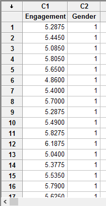
In Minitab, we set up the two variables. Under column we entered the name of the dependent variable, Engagement, as follows: . Then, under column we entered the name of the independent variable, Gender, as follows: . Finally, we entered the scores on the dependent and independent variable into the Engagement and Gender columns, respectively. For the independent variable, Gender, we gave "Males" a value of "1" and "Females" a value of "2". This data setup in Minitab is illustrated below:

Published with written permission from Minitab Inc.

Note: If you do not have all the data for your two variables, unlike our example above, but only the summarized data (e.g., the sample size, mean and standard deviation of the dependent variable for each of the two groups of your independent variable), you will need to set up your data differently.

Minitab

Test Procedure in Minitab

In this section, we show you how to analyse your data using an independent t-test in Minitab when the six assumptions in the previous section, Assumptions, have not been violated. Therefore, the three steps required to run an independent t-test in Minitab are shown below:

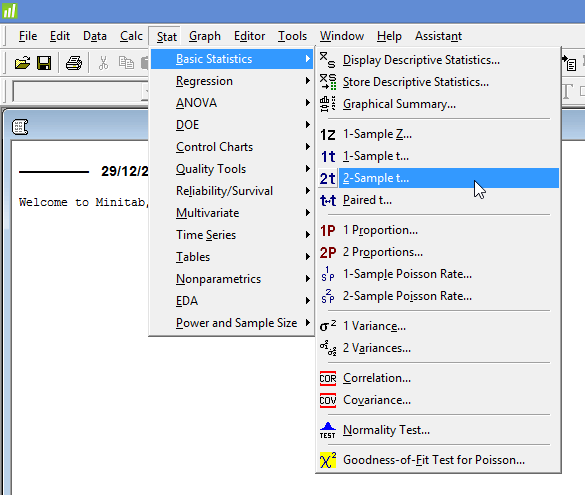
1. Click Stat > Basic Statistics > 2-Sample t... on the top menu, as shown below:
   

   Published with written permission from Minitab Inc.

   
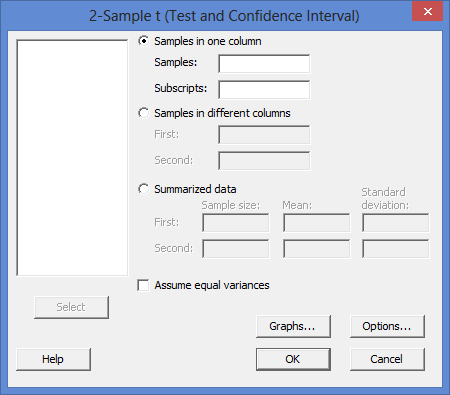
   You will be presented with the following 2-Sample t (Test and Confidence Interval) dialogue box:
   
   

   Published with written permission from Minitab Inc.

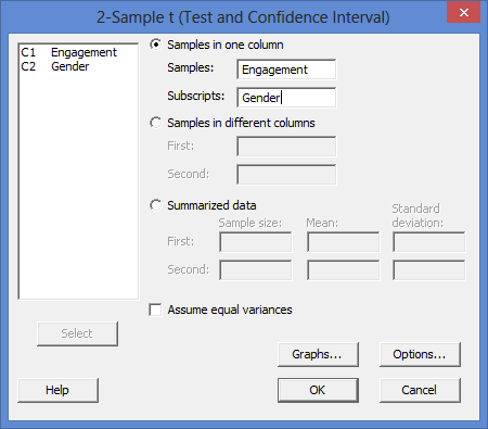
2. Leave the Samples in one column option selected. Then, enter the dependent variable, Engagement, into the Samples: box, and the independent variable, Gender, into the Subscripts: box. You will end up with the dialogue box shown below:
   

   Published with written permission from Minitab Inc.

   Note 1: To transfer your variables, you first need to click into the Samples: box for your two variables to appear in the main left-hand box (e.g., C1   Engagement and C2   Gender). This will activate the button (it is usually faded: ). To transfer the dependent variable, Engagement, into the Samples: box, you can now either select C1   Engagement in the main left-hand box and press the button or simply double-click on C1   Engagement. You now need to do the same for C2   Gender, but this time into the Subscripts: box.

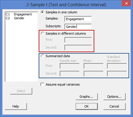
   Explanation: In addition to the procedure above, there are two other methods for carrying out an independent t-test in Minitab (one using the options highlighted in the red rectangle below and the other the options highlighted in the blue rectangle).
   
   
   
   The first (in the red rectangle) is useful if you have all the scores in your data set (e.g., the scores for each of the 40 participants in our example), but you have entered your data into Minitab in a different way to the one shown in the Setup in Minitab section earlier. The second (in the blue rectangle) is useful if you only have the summarized data (e.g., the sample size, mean and standard deviation of the dependent variable for each of the two groups of your independent variable), rather than all the scores.

   Note 2: By default, Minitab uses 95% confidence intervals, which equates to declaring statistical significance at the p < .05 level. If you want to change this, you can do so by first clicking on the button, which opens the 2-Sample t - Options dialogue box, as shown below:
   
   
   
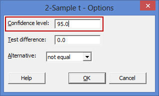
   To change the value of the confidence interval, simply click into the Confidence level: box – highlighted in red above – and change the value (e.g., a value of 99.0 would equate to declaring statistical significance at the p < .01 level).

3. Click on the button. The output that Minitab produces is shown below.

Minitab

Output of the independent t-test in Minitab

The Minitab output for the independent t-test is shown below. This output provides useful descriptive statistics for the two independent groups that were compared, including the sample size, mean, standard deviation and standard error of the mean, as well as actual results from the independent t-test.

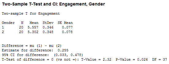
Looking at the "Mean" column, you can see that mean engagement scores were higher for males (coded 1 in the "Gender" column) compared to females (coded 2 in the "Gender" column). The mean difference in engagement between the two groups (i.e., males and females) was 0.255 (the Estimate for difference row) with 95% confidence intervals (95% CI) for the mean difference in engagement of 0.033 to 0.478 (the 95% CI for difference row). You are also presented with the degrees of freedom (DF), which are 37, an obtained t-value (T-Value) of 2.32 and the statistical significance (2-tailed p-value) of the independent t-test (P-Value), which is 0.026. As the p-value is less than 0.05 (i.e., p < .05), it can be concluded that there is a statistically significant difference in mean engagement between our two groups: males and females. In other words, the mean difference in engagement between males and females is not equal to zero.

Note: We present the output from the independent t-test above. However, since you should have tested your data for the assumptions we explained earlier in the Assumptions section, you will also need to interpret the Minitab output that was produced when you tested for them. This includes: (a) the boxplots you used to check if there were any significant outliers; (b) the output Minitab produces for your Shapiro-Wilk test of normality to determine normality; and (c) the output Minitab produces for Levene's test for homogeneity of variances. Also, remember that if your data failed any of these assumptions, the output that you get from the independent t-test procedure (i.e., the output we discuss above) might no longer be valid, and you will need to interpret the alternative Minitab output that is produced when they fail (i.e., this includes different results).

Minitab

Reporting the output of the independent t-test

When you report the output of your independent t-test, it is good practice to include:

• A. An introduction to the analysis you carried out.
• B. Information about your sample (N), including how many participants were in each of your two groups (N.B., this is particularly useful if the group sizes were unequal or there were missing values).
• C. A statement of whether there was a statistically significant difference between your two groups, including the relevant means (Mean) and standard deviations (StDev), mean difference (Estimate for difference), 95% confidence interval for the mean difference (95% CI for difference), t-value (T-Value), degrees of freedom (DF), and significance level, or more specifically, the 2-tailed p-value (P-Value).

Based on the Minitab output above, we could report the results of this study as follows:

In addition to the reporting the results as above, a diagram can be used to visually present your results. For example, you could do this using a bar chart with error bars (e.g., where the errors bars could be the standard deviation, standard error or 95% confidence intervals). This can make it easier for others to understand your results. Furthermore, you are increasingly expected to report an "effect size" in addition to your independent t-test results. Effect sizes are important because whilst the independent t-test tells you whether the difference between group means is "real" (i.e., different in the population), it does not tell you the "size" of the difference. Whilst Minitab will not produce these effect sizes for you using this procedure, there is a procedure in Minitab to do so.

Portions of information contained in this publication/book are printed with permission of Minitab Inc. All such material remains the exclusive property and copyright of Minitab Inc. All rights reserved.