Mann-Whitney U test using Minitab

Introduction

The Mann-Whitney U test determines whether there is a statistically significant difference between two unrelated, independent groups on a dependent variable.

For example, you could use a Mann-Whitney U test to determine whether there is a difference in test anxiety between undergraduate and postgraduate students (i.e., the dependent variable would be "test anxiety", and the independent variable would be "educational level", which has two groups: "undergraduate students" and "postgraduate students"). Alternately, you could use a Mann-Whitney U test to determine whether there is a difference in typing speed based on room lighting (i.e., the dependent variable would be "typing speed" and the independent variable would be "room lighting", which has two groups: "red lighting" and "blue lighting").

In this guide, we show you how to carry out a Mann-Whitney U test using Minitab, as well as interpret and report the results from this test. However, before we introduce you to this procedure, you need to understand the different assumptions that your data must meet in order for a Mann-Whitney U test to give you a valid result. We discuss these assumptions next.

Minitab

Assumptions

The Mann-Whitney U test has four "assumptions". You cannot test the first three of these assumptions with Minitab because they relate to your study design and choice of variables. However, you should check whether your study meets these three assumptions before moving on. If these assumptions are not met, there is likely to be a different statistical test that you can use instead. Assumptions #1, #2 and #3 are explained below:

• Assumption #1: Your dependent variable should be measured at a continuous (i.e., they are interval or ratio variables) or ordinal level. Examples of continuous variables include height (measured in feet and inches), temperature (measured in ^oC), salary (measured in US dollars), revision time (measured in hours), intelligence (measured using IQ score), firm size (measured in terms of the number of employees), age (measured in years), reaction time (measured in milliseconds), grip strength (measured in kg), power output (measured in watts), test performance (measured from 0 to 100), sales (measured in number of transactions per month), academic achievement (measured in terms of GMAT score), and so forth. Examples of ordinal variables include Likert items (e.g., a 7-point scale from "strongly agree" through to "strongly disagree"), amongst other ways of ranking categories (e.g., a 5-point scale explaining how much a customer liked a product, ranging from "Not very much" to "Yes, a lot"). If you are unsure whether your dependent variable is continuous (i.e., measured at the interval or ratio level) or ordinal, see our Types of Variable guide.
• Assumption #2: Your independent variable should consist of two categorical, independent (unrelated) groups. Examples of such independent variables include gender (two groups: male or female), treatment type (two groups: medication or no medication), educational level (two groups: undergraduate or postgraduate), health insurance (two groups: yes or no), intensity of religious practice (two groups: practicing or non-practicing), personality type (two groups: introversion or extroversion), and so forth.
• Assumption #3: You should have independence of observations, which means that there is no relationship between the observations in each group or between the groups themselves. Therefore, there must be different participants in each group with no participant being in more than one group. For example, if you wanted to determine whether there was a statistically significant difference in anxiety level between undergraduates and postgraduates (i.e., your two independent groups), a participant cannot be both an undergraduate and a postgraduate. The participant can only be an undergraduate or a postgraduate. The participant cannot be in both groups. If you do not have independence of observations, it is likely you have "related groups", which means you will probably need to use a Wilcoxon signed-rank test instead of the Mann-Whitney U test (see our Wilcoxon signed-rank test in Minitab guide).

Assumption #4 relates to the nature of your data and can be checked using Minitab. You have to check that your data meets this assumption because if it does not, the results you get when running a Mann-Whitney U test might not be valid. In fact, do not be surprised if your data violates this assumption. This is not uncommon. However, there are possible solutions such that you can still use a Mann-Whitney U test. Assumption #4 is explained below:

• Assumption #4: A Mann-Whitney U test can be used when your two variables are not normally distributed. However, for a Mann-Whitney U test to be able to provide a valid test of the difference between two medians, both distributions must be the same shape (e.g., the distribution of the scores for "males" and the distributions of the scores for "females" must have the same shape). When you analyze your own data, it is extremely unlikely that your two distributions will be identical, but they may have the same (or a 'similar') shape. If they do have the same shape, you can use Minitab to carry out a Mann-Whitney U test to compare the medians of your dependent variable for the two groups of the independent variable you are interested in (e.g., the medians of engagement score for males and females). However, if your two distributions have a different shape, you can only use the Mann-Whitney U test to compare mean ranks. This is something that you can test for using Minitab.

In practice, checking for assumption #4 will probably take up most of your time when carrying out a Mann-Whitney U test. However, it is not a difficult task, and Minitab provides all the tools you need to do this.

In the section, Test Procedure in Minitab, we illustrate the Minitab procedure required to perform a Mann-Whitney U test assuming that no assumptions have been violated. First, we set out the example we use to explain the Mann-Whitney U test procedure in Minitab.

Minitab

Example

A company commissions an Advertising Agency to create a TV advert to promote a new product. Since the product is designed for men and women, the TV advert has to appeal to men and women equally. Before the company spends $250,000 to run the advert across a number of TV networks, it wants to make sure that it appeals equally to men and women. More specifically, the company wants to know whether the way that men and women "engage" with the TV advert is the same.

To achieve this, the TV advert is shown to 20 men and 20 women, who are then asked to fill in a questionnaire that measures their engagement with the advertisement. The questionnaire provides an overall engagement score. This overall engagement score is the dependent variable, which we have labelled Engagement in Minitab. Our independent variable, which we have labelled Gender in Minitab, contains two groups: "Males" and "Females".

An independent t-test was used to determine whether there was a statistically significant difference in mean engagement between males and females. Since the Advertising Agency needs the advertisement to be similarly engaging, they hope there is no difference!

Minitab

Setup in Minitab

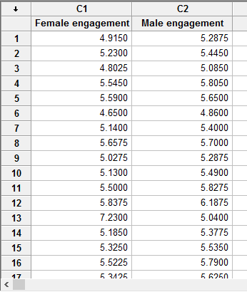
In Minitab, we set up the two related groups as though they were two variables. Therefore, under column we entered the name of the first related group, Female engagement, as follows: . Then, under column we entered the name of the second related group, Male engagement, as follows: . Finally, we entered the scores on the dependent variable for each of the two independent groups (i.e., the engagement score for "females" in the Female engagement column and the engagement scores for "males" in the Male engagement column). This is illustrated below:

Published with written permission from Minitab Inc.

Minitab

Test Procedure in Minitab

In this section, we show you how to analyze your data using a Mann-Whitney U test in Minitab when the four assumptions in the previous section, Assumptions, have not been violated. Therefore, the three steps required to run a Mann-Whitney U test in Minitab are shown below:

1. Click Stat > Nonparametrics > Mann-Whitney... on the top menu, as shown below:
   

   Published with written permission from Minitab Inc.

   
   You will be presented with the following Mann-Whitney dialogue box:
   
   

   Published with written permission from Minitab Inc.

2. Enter Female engagement in the First Sample: box and Male engagement into the Second Sample: box. You will end up with the dialogue box shown below:
   

   Published with written permission from Minitab Inc.

   Note 1: To transfer your variables, you first need to click inside the First Sample: box for your two groups to appear in the main left-hand box (e.g., C1   Female engagement and C2   Male engagement). This will activate the button (it is usually faded: ). To transfer the first group, Female engagement, into the First Sample: box, you can now either select C1   Female engagement in the main left-hand box and press the button or simply double-click on C1   Female engagement. You now need to do the same for C2   Male engagement, but this time into the Second Sample: box.

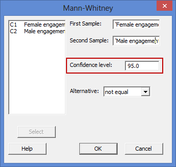
   Note 2: By default, Minitab uses 95% confidence intervals, which equates to declaring statistical significance at the p < .05 level. If you want to change the value of the confidence interval, simply enter the new value into the Confidence level: box (e.g., a value of 99.0 would equate to declaring statistical significance at the p < .01 level), highlighted in red below:
   
   

3. Click on the button. The output that Minitab produces is shown below.

Minitab

Output of the Mann-Whitney U test in Minitab

The Minitab output for the Mann-Whitney U test is shown below. This output provides useful descriptive statistics for the two independent groups that were compared, including the sample size and median, as well as actual results from the Mann-Whitney U test.

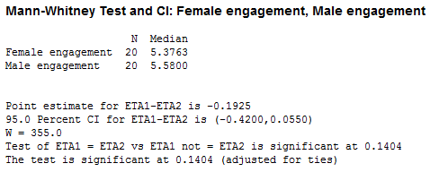
Looking at the "Median" column, you can see that median engagement scores were higher for males (the Male engagement row) compared to females (the Female engagement row). The median difference in engagement between the two groups (i.e., males and females) was -0.1925 (the Point estimate for ETA1-ETA2 row) with 95% confidence intervals (95% CI) for the median difference in engagement of -0.420 to 0.055 (the 95.0 Percent CI for ETA1-ETA2 row) (ETA is the name given to the median). You are also presented with the Wilcoxon test statistic, W (W) of 355.0 and the statistical significance (2-tailed p-value) of this test (the Test of ETA1 = ETA2 vs ETA1 not = ETA2 is significant row), which is 0.1404 (the p-value is adjusted for ties and is equivalent to the Mann-Whitney U test). As the p-value is greater than 0.05 (i.e., p > .05), it can be concluded that there isn't a statistically significant difference in median engagement between our two groups: males and females. In other words, the median difference in engagement between males and females is not statistically significantly different l to zero.

Note: We present the output from the Mann-Whitney U test above. However, since you should have tested your data for the assumptions we explained earlier in the Assumptions section, you will also need to interpret the Minitab output that was produced when you tested for them. This includes the histograms that are produced to determine whether the two distributions of your independent variable (e.g., the distributions for "males" and "females") have the same shape. Also, remember that if your data failed any of these assumptions, the output that you get from the Mann-Whitney U test procedure (i.e., the output we discuss above) might no longer be valid.

Minitab

Reporting the output of the Mann-Whitney U test

When you report the output of your Mann-Whitney U test, it is good practice to include:

• A. An introduction to the analysis you carried out.
• B. Information about your sample (N), including how many participants were in each of your two groups (N.B., this is particularly useful if the group sizes were unequal or there were missing values).
• C. A statement of whether there was a statistically significant difference between your two groups, including the relevant medians (Median), the Mann-Whitney U statistic if available, and the significance level, or more specifically, the 2-tailed p-value (i.e., the value at the end of the Test of ETA1 = ETA2 vs ETA1 not = ETA2 is significant row).

Based on the Minitab output above, we could report the results of this study as follows:

Portions of information contained in this publication/book are printed with permission of Minitab Inc. All such material remains the exclusive property and copyright of Minitab Inc. All rights reserved.