One-way ANOVA using Stata

Introduction

The one-way analysis of variance (ANOVA) is used to determine whether the mean of a dependent variable is the same in two or more unrelated, independent groups. However, it is typically only used when you have three or more independent, unrelated groups, since an independent-samples t-test is more commonly used when you have just two groups. If you have two independent variables you can use a two-way ANOVA. Alternatively, if you have multiple dependent variables you can consider a one-way MANOVA.

For example, you can use a one-way ANOVA to determine whether exam performance differed based on test anxiety levels amongst students (i.e., your dependent variable would be "exam performance", measured from 0-100, and your independent variable would be "test anxiety levels", which has three groups: "low stressed students", "medium stressed students, and "high stressed students"). Alternately, a one-way ANOVA could be used to understand whether there is a difference in salary based on degree type (i.e., your dependent variable would be "salary" and your independent variable would be "degree type", which has five groups: "business studies", "psychology", "biological sciences", "engineering" and "law").

When there is a statistically significant difference between the groups, it is possible to determine which specific groups were significantly different from each other using post hoc tests. You need to conduct these post hoc tests because the one-way ANOVA is an omnibus test and cannot tell you which specific groups were significantly different from each other; it only tells you that at least two groups were different.

This "quick start" guide shows you how to carry out a one-way ANOVA with post hoc tests using Stata, as well as how to interpret and report the results from this test. However, before we introduce you to this procedure, you need to understand the different assumptions that your data must meet in order for a one-way ANOVA to give you a valid result. We discuss these assumptions next.

Stata

Assumptions

There are six "assumptions" that underpin the one-way ANOVA. If any of these six assumptions are not met, you cannot analyse your data using a one-way ANOVA because you will not get a valid result. Since assumptions #1, #2 and #3 relate to your study design and choice of variables, they cannot be tested for using Stata. However, you should decide whether your study meets these assumptions before moving on.

• Assumption #1: Your dependent variable should be measured at the continuous level. Examples of such continuous variables include height (measured in feet and inches), temperature (measured in °C), salary (measured in US dollars), revision time (measured in hours), intelligence (measured using IQ score), reaction time (measured in milliseconds), test performance (measured from 0 to 100), sales (measured in number of transactions per month), and so forth. If you are unsure whether your dependent variable is continuous (i.e., measured at the interval or ratio level), see our Types of Variable guide. If your dependent variable is ordinal, you might consider running a Kruskal-Wallis H test instead.
• Assumption #2: Your independent variable should consist of two or more categorical, independent (unrelated) groups. Examples of categorical variables include gender (e.g., 2 groups: male and female), ethnicity (e.g., 3 groups: Caucasian, African American and Hispanic), physical activity level (e.g., 4 groups: sedentary, low, moderate and high), and profession (e.g., 5 groups: surgeon, doctor, nurse, dentist, therapist).
• Assumption #3: You should have independence of observations, which means that there is no relationship between the observations in each group or between the groups themselves. For example, there must be different participants in each group with no participant being in more than one group. If you do not have independence of observations, it is likely you have "related groups", which means you will need to use a one-way repeated measures ANOVA instead of the one-way ANOVA .

Fortunately, you can check assumptions #4, #5 and #6 using Stata. When moving on to assumptions #4, #5 and #6, we suggest testing them in this order because it represents an order where, if a violation to the assumption is not correctable, you will no longer be able to use a one-way ANOVA. In fact, do not be surprised if your data fails one or more of these assumptions since this is fairly typical when working with real-world data rather than textbook examples, which often only show you how to carry out a one-way ANOVA when everything goes well. However, don’t worry because even when your data fails certain assumptions, there is often a solution to overcome this (e.g., transforming your data or using another statistical test instead). Just remember that if you do not check that you data meets these assumptions or you test for them correctly, the results you get when running a one-way ANOVA might not be valid.

• Assumption #4: There should be no significant outliers. An outlier is simply a single case within your data set that does not follow the usual pattern (e.g., in a study of 100 students' IQ scores, where the mean score was 108 with only a small variation between students, one student had a score of 156, which is very unusual, and may even put her in the top 1% of IQ scores globally). The problem with outliers is that they can have a negative effect on the one-way ANOVA, reducing the accuracy of your results. Fortunately, when using Stata to run a one-way ANOVA on your data, you can easily detect possible outliers.
• Assumption #5: Your dependent variable should be approximately normally distributed for each category of the independent variable. Your data need only be approximately normal for running a one-way ANOVA because it is quite "robust" to violations of normality, meaning that this assumption can be a little violated and still provide valid results. You can test for normality using the Shapiro-Wilk test of normality, which is easily tested for using Stata.
• Assumption #6: There needs to be homogeneity of variances. You can test this assumption in Stata using Levene's test for homogeneity of variances. Levene's test is very important when it comes to interpreting the results from a one-way ANOVA guide because Stata is capable of producing different outputs depending on whether your data meets or fails this assumption.

In practice, checking for assumptions #4, #5 and #6 will probably take up most of your time when carrying out a one-way ANOVA. However, it is not a difficult task, and Stata provides all the tools you need to do this.

In the section, Test Procedure in Stata, we illustrate the Stata procedure required to perform a one-way ANOVA assuming that no assumptions have been violated. First, we set out the example we use to explain the one-way ANOVA procedure in Stata.

Stata

Example

An online retailer wants to get the best from employees, as well as improve their working experience. Currently, employees in the retailer’s order fulfilment centre are not provided with any kind of entertainment whilst they work (e.g., background music, television, etc.). However, the retailer wants to know whether providing music, which a few employees have requested, would lead to greater productivity, and if so, by how much.

Therefore, the researcher recruit a random sample of 60 employees. This sample of 60 participants was randomly split into three independent groups with 20 participants in each group: (a) a "control group" that did not listen to music; (b) a "treatment group" who listened to music, but had no choice of what they listened to; and (c) a second treatment group who listened to music and had a choice of what they listened to.

The experiment lasted for one month. At the end of the experiment, the "productivity" of the three groups was measured in terms of the "average number of packages processed per hour". Therefore, the dependent variable was "productivity" (measured in terms of the average number of packages processed per hour during the one month experiment), whilst the independent variable was "treatment type", where there were three independent groups: "No music" (control group), "Music - No choice" (treatment group A) and "Music - Choice" (treatment group B).

A one-way ANOVA was used to determine whether there was a statistically significant difference in productivity between the three independent groups.

Note: The example and data used for this guide are fictitious. We have just created them for the purposes of this guide.

Stata

Setup in Stata

In Stata, we separated the three groups for analysis by creating the independent variable, called Music, and gave: (a) a value of "1 -- No music" to the control group; (b) a value of "2 -- Music - No choice" to the treatment group who listened to music, but had no choice of what they listened to; and (c) a value of "3 -- Music - Choice" to the treatment group who listened to music and had a choice of what they listened to, as shown below:

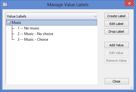
Published with written permission from StataCorp LP.

The scores for the independent variable, Music, were then entered into the left-hand column of the Data Editor (Edit) spreadsheet, whilst the values for the dependent variable, Productivity, were entered into the right-hand column, as shown below:

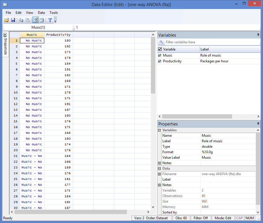
Published with written permission from StataCorp LP.

Stata

Test Procedure in Stata

In this section, we show you how to analyse your data using a one-way ANOVA in Stata when the six assumptions in the previous section, Assumptions, have not been violated. You can carry out a one-way ANOVA using code or Stata's graphical user interface (GUI). After you have carried out your analysis, we show you how to interpret your results. First, choose whether you want to use code or Stata's graphical user interface (GUI).

Stata

Code

In the first section below, we set out the code to carry out a one-way ANOVA, and in the second section, the post hoc test that follows the one-way ANOVA. All code is entered into Stata's box, as illustrated below:

Published with written permission from StataCorp LP.

One-way ANOVA

The code to run a one-way ANOVA on your data takes the form:

oneway DependentVariable IndependentVariable, tabulate

Using our example where the dependent variable is Productivity and the independent variable is Music, the required code would be:

oneway Productivity Music, tabulate

Note: You can run the oneway command without adding the tabulate command to the end of the code, but this provides useful descriptive statistics (i.e., the mean, standard deviation and N), so we choose to include it.

Therefore, enter the code and press the "Return/Enter" button on your keyboard.

You can see the Stata output that will be produced here. If there is a statistically significant difference between your groups, you can then carry out post hoc tests using the code below to determine where any differences lie.

Post hoc testing

There are many types of post hoc test that you can use following a one-way ANOVA (e.g., Bonferroni, Sidak, Scheffe, Tukey, etc.). We show you the code to run the Tukey post hoc test below, which takes the form:

pwmean DependentVariable, over[IndependentVariable], mcompare(tukey) effects

Using our example where the dependent variable is Productivity and the independent variable is Music, the required code would be:

pwmean Productivity, over[Music], mcompare(tukey) effects

Note: You need to run the one-way ANOVA in Stata before you can carry out post hoc tests or Stata will display the following error message: "last estimates not found". It is not enough that your file is set up correctly with the relevant dependent and independent variables correctly labelled. Stata doesn't identify these for the purposes of carrying out post hoc tests until you have first run the one-way ANOVA. Therefore, if you get an error message, you will have to run the one-way ANOVA procedure again and then enter the post hoc code a second time.

Therefore, enter the code and press the "Return/Enter" button on your keyboard.

You can see the Stata output that will be produced from the post hoc test here and the main one-way ANOVA procedure here.

Stata

Graphical User Interface (GUI)

In the first section below, we set out the code to carry out a one-way ANOVA, and in the second section, the post hoc test that follows the one-way ANOVA.

One-way ANOVA

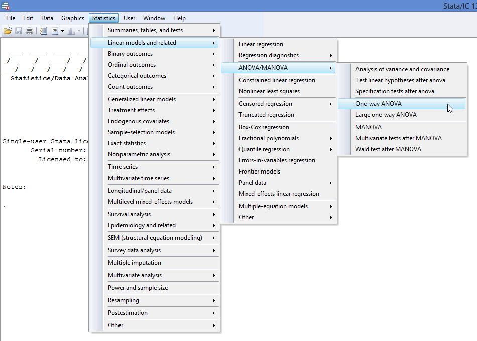
1. Select Statistics > Linear models and related > ANOVA/MANOVA > One-way ANOVA on the top menu, as shown below:
   

   Published with written permission from StataCorp LP.

   
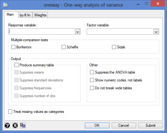
   You will be presented with the following oneway - One-way analysis of variance dialogue box:
   
   

   Published with written permission from StataCorp LP.

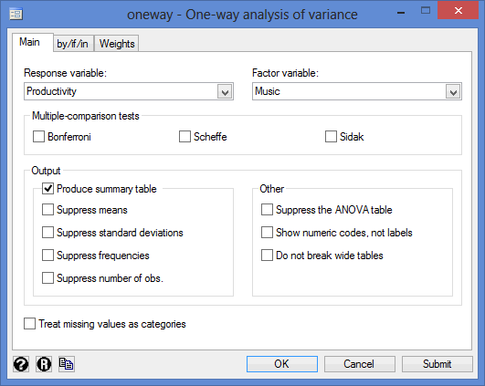
2. Select the dependent variable, Productivity, from within the Response variable: drop-down box, and the independent variable, Music, in the Factor variable: drop-down box. Next, tick the Produce summary table box in the –Output– area, as shown below:
   

   Published with written permission from StataCorp LP.

3. Click on the button.

You can see the Stata output that will be produced here. If there is a statistical significant difference between your groups, you can then carry out post hoc tests using the procedure below to determine where any differences lie.

Post hoc tests

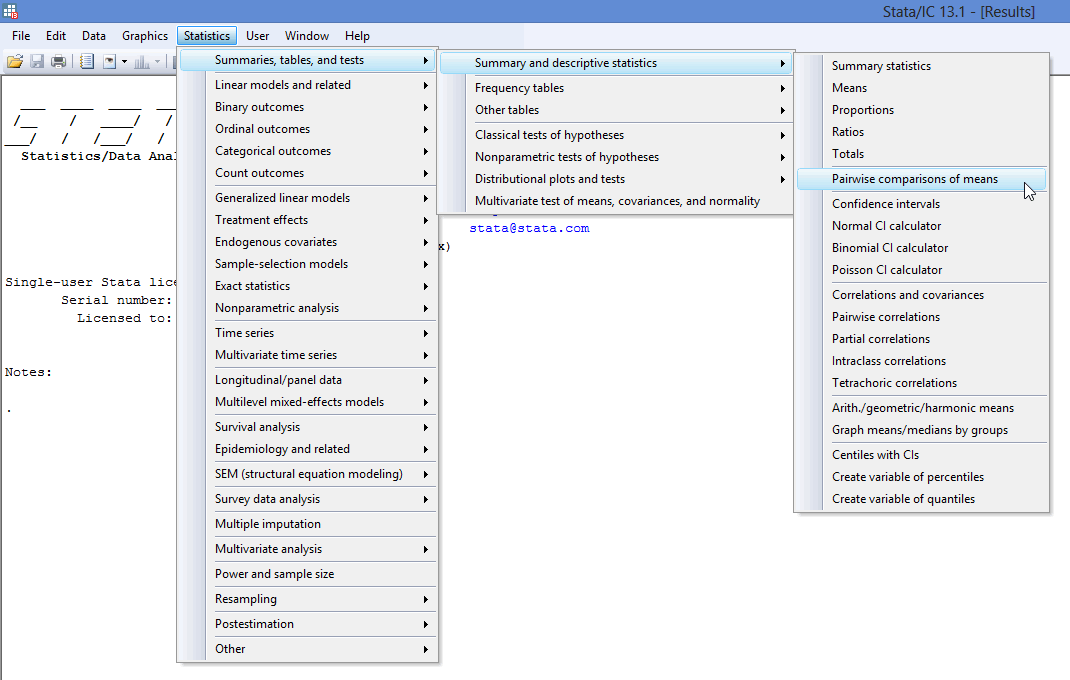
1. Click Statistics > Summaries, tables, and tests > Summary and descriptive statistics > Pairwise comparisons of means on the top menu, as shown below:
   

   Published with written permission from StataCorp LP.

   
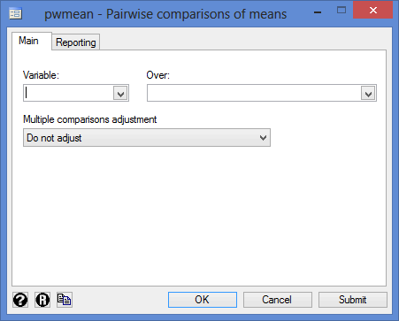
   You will be presented with the following pwmean - Pairwise comparisons of means dialogue box:
   
   

   Published with written permission from StataCorp LP.

2. Select the dependent variable, Productivity, from within the Variable: drop-down box, and the independent variable, Music, from within the Over: drop-down box. Next, select the post-hoc test from within the Multiple comparisons adjustment drop down box, as shown below:
   

   Published with written permission from StataCorp LP.

   Note: You need to run the one-way ANOVA in Stata before you can carry out post hoc tests or Stata will show an error message. It is not enough that your file is set up correctly with the relevant dependent and independent variables correctly labelled. Stata doesn't identify these for the purposes of carrying out post hoc tests until you have first run the one-way ANOVA. Therefore, if you get an error message, you will have to run the one-way ANOVA procedure again and then follow the post hoc procedure for a second time.

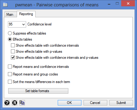
3. Click on the tab highlighted in the red rectangle. You will end up with a screen similar to the one below:
   

   Published with written permission from StataCorp LP.

4. Keep the default 95% confidence interval by not changing the 95 value in the Confidence level drop-down box. Next, select the Effects tables option, which will open up three further options below. Finally, tick the Show effects table with confidence intervals and p-values box, as shown below:
   

   Published with written permission from StataCorp LP.

5. Click on the button.

You can see the Stata output that will be produced from the post hoc test here and the main one-way ANOVA procedure here.

Stata

Output of the One-Way ANOVA in Stata

If your data passed assumption #4 (i.e., there were no significant outliers), assumption #5 (i.e., your dependent variable was approximately normally distributed for each group of the independent variable) and assumption #6 (i.e., there was homogeneity of variances), which we explained earlier in the Assumptions section, you will only need to interpret the following Stata output for the one-way ANOVA:

Stata

Descriptive statistics

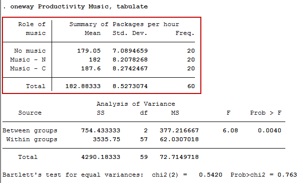
The descriptives output, highlighted in the red rectangle below, provides some very useful descriptive statistics, including the mean, standard deviation and sample sizes for the dependent variable (Productivity) for each group of the independent variable, Music (i.e., "No music", "Music - No choice" and "Music - Choice"), as well as when all groups are combined (Total). These figures are useful when you need to describe your data.

Published with written permission from StataCorp LP.

Stata

One-way ANOVA results

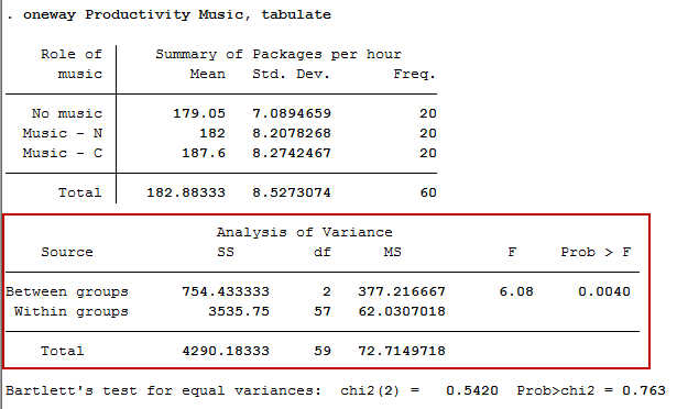
The Stata output for the one-way ANOVA is shown in the red rectangle below, indicating whether we have a statistically significant difference between our three group means. We can see that the significance level is 0.0040 (p = .004), which is below 0.05. and, therefore, there is a statistically significant difference in the mean productivity between the three different groups of the independent variable, Music (i.e., "No Music", "Music - No Choice" and "Music - Choice"). This is great to know, but we do not know which of the specific groups differed. Luckily, we can find this out in the Pairwise comparisons of means with equal variances output that contains the results of our post hoc tests (see below).

Published with written permission from StataCorp LP.

Stata

Pairwise comparisons results for the Tukey post hoc test

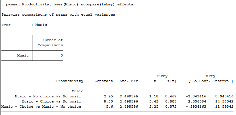
From the results so far, we know that at least one of the group means is different from the other group means. Next, we can use the Stata output below, entitled Pairwise comparisons of means with equal variances, to determine which groups differed from each other. Looking at the p-value (i.e., the P>|t| row under the Tukey column), we can see that there is a statistically significant difference in productivity between the "Music - Choice" group who listened to music (and had a choice over what music they listened to) and the "No music" control group who did not listen to music (p = 0.003). However, there were no differences between the "Music - No choice" group who listened to music (but had no choice over what music they listened to) and the "No music" control group (p = 0.467), or between the "Music - Choice" group and "Music - No choice" group (p = 0.072).

Published with written permission from StataCorp LP.

In the section that follows, we show you how you could report these results.

Note: We present the output from the one-way ANOVA above. However, since you should have tested your data for the assumptions we explained earlier in the Assumptions section, you will also need to interpret the Stata output that was produced when you tested for them. This includes: (a) the boxplots you used to check if there were any significant outliers; (b) the output Stata produces for your Shapiro-Wilk test of normality to determine normality; and (c) the output Stata produces for Levene's test for homogeneity of variances. Also, remember that if your data failed any of these assumptions, the output that you get from the one-way ANOVA procedure (i.e., the output we discuss above) will no longer be relevant, and you will need to interpret the Stata output that is produced when they fail (i.e., this includes different results).

Stata

Reporting the Output of the One-Way ANOVA

When you report the output of your one-way ANOVA, it is good practice to include:

• A. An introduction to the analysis you carried out.
• B. Information about your sample (including how many participants were in each of your groups if the group sizes were unequal or there were missing values).
• C. A statement of whether there were statistically significant differences between your groups (including the observed F-value [F], degrees of freedom [df], and significance level, or more specifically, the 2-tailed p-value [Prob > F].
• D. If there was a statistically significant difference between the groups, the results from the Tukey post hoc test, including the mean (Contrast) and standard error (Std. Err.) for each of your groups, as well as the relevant 2-tailed p-value [Prob > |t|].

Based on the Stata output above, we could report the results of this study as follows:

In addition to the reporting the results as above, a diagram can be used to visually present your results. For example, you could do this using a bar chart with error bars (e.g., where the errors bars could be the standard deviation, standard error or 95% confidence intervals). This can make it easier for others to understand your results. Furthermore, you are increasingly expected to report "effect sizes" in addition to your one-way ANOVA results. Effect sizes are important because whilst the one-way ANOVA tells you whether differences between group means are "real" (i.e., different in the population), it does not tell you the "size" of the difference. Whilst Stata will not produce these effect sizes for you using this procedure, there is a procedure in Stata to do so.