One-Way Repeated Measures ANOVA using Stata

Introduction

A one-way repeated measures ANOVA (also known as a within-subjects ANOVA) is used to determine whether three or more group means are different where the participants are the same in each group. For this reason, the groups are sometimes called "related" groups. You will most often come across this situation for two reasons: (a) participants have been measured over multiple time points to see if there have been any changes, usually in response to an intervention; or (b) participants have been subjected to more than one condition/trial and the response to each of these conditions is to be compared.

For example, you could use a one-way repeated measures ANOVA to understand whether there is a difference in anxiety levels amongst moderately anxious participants after a hypnotherapy programme aimed at reducing anxiety (e.g., with three time points: anxiety immediately before, 1 month after and 6 months after the hypnotherapy programme). In this example, "anxiety level" is your dependent variable, whilst your independent variable is "time" (i.e., with three related groups, where each of the three time points is considered a "related group"). Alternately, you could use a one-way repeated measures ANOVA to understand whether there is a difference in downhill skiing performance based on three different coloured tints of ski goggles (e.g., ski performance under three conditions: wearing brown, blue and red tinted ski goggles). In this example, "ski performance" is your dependent variable, whilst your independent variable is "condition" (i.e., with three related groups, where each of the three conditions is considered a "related group").

In this guide, we show you how to carry out a one-way repeated measures ANOVA using Stata, as well as interpret and report the results from this test. However, before we introduce you to this procedure, you need to understand the different assumptions that your data must meet in order for a one-way repeated measures ANOVA to give you a valid result. We discuss these assumptions next.

Stata

Assumptions

There are five assumptions that underpin the one-way repeated measures ANOVA. If any of these five assumptions are not met, you might not be able to analyse your data using a one-way repeated measures ANOVA because you might not get a valid result. Since assumptions #1 and #2 relate to your study design and choice of variables, they cannot be tested for using Stata. However, you should decide whether your study meets these assumptions before moving on.

• Assumption #1: Your dependent variable should be measured at the interval or ratio level (i.e., it is a continuous variable). Examples of continuous variables include revision time (measured in hours), intelligence (measured using IQ score), exam performance (measured from 0 to 100), weight (measured in kg), and so forth. You can learn more about interval and ratio variables in our article: Types of Variable.
• Assumption #2: Your independent variable (also known as the within-subjects factor) should consist of at least two categorical, "related groups". "Related groups" indicates that the same subjects are present in all groups. The reason it is possible to have the same subjects in each group is because each subject has been measured on two or more occasions on the same dependent variable. For example, you might have measured 10 individuals' performance in a spelling test (the dependent variable) before, at the mid point, and after they underwent a new form of computerized teaching method to improve spelling. The first related group consists of the subjects at the beginning (prior to) the computerized spelling training, the second at the mid point of training, and the third and final related group consists of the same subjects, but now at the end of the computerized training. These repeated measurements (i.e., related groups) are also referred to as levels of the within-subjects factor. The repeated measures ANOVA can also be used to compare different subjects, but this does not happen very often.

Fortunately, you can check assumptions #3, #4 and #5 using Stata. However, do not be surprised if your data fails one or more of these assumptions since this is fairly typical when working with real-world data rather than textbook examples, which often only show you how to carry out a one-way repeated measures ANOVA when everything goes well. However, don’t worry because even when your data fails certain assumptions, there can be a solution to overcome this (e.g., transforming your data or using another statistical test instead). Just remember that if you do not check that your data meets these assumptions or you test for them incorrectly, the results you get when running a one-way repeated measures ANOVA might not be valid.

• Assumption #3: There should be no significant outliers in any of the related groups (i.e., in any levels of the within-subjects factor). An outlier is simply a single data point within your data that does not follow the usual pattern (e.g., in a study of 100 students' IQ scores, where the mean score was 108 with only a small variation between students, one student had a score of 156, which is very unusual, and may even put her in the top 1% of IQ scores globally). There can be multiple outliers. The problem with outliers is that they can have a negative effect on the repeated measures ANOVA, reducing the accuracy of your results. Fortunately, when using Stata to run a one-way repeated measures ANOVA on your data, you can easily detect possible outliers.
• Assumption #4: The distribution of the dependent variable in the two or more related groups should be approximately normally distributed. We talk about the repeated measures ANOVA only requiring approximately normal data because it is quite "robust" to violations of normality, meaning that the assumption can be a little violated and still provide valid results. You can test for normality using the Shapiro-Wilk test for normality, which can be easily performed in Stata.
• Assumption #5: Known as sphericity, the variances of the differences between all combinations of related groups must be equal. Unfortunately, the one-way repeated measures ANOVA is particularly susceptible to violating the assumption of sphericity, which causes the test to become too liberal (i.e., leads to an increase in the Type I error rate; that is, the likelihood of detecting a statistically significant result when there isn't one).

In practice, checking for assumptions #3, #4 and #5 will probably take up most of your time when carrying out a one-way repeated measures ANOVA. However, it is not a difficult task, and Stata provides all the tools you need to do this.

In the section, Test Procedure in Stata, we illustrate the Stata procedure required to perform a one-way repeated measures ANOVA assuming that no assumptions have been violated. First, we set out the example we use to explain the one-way repeated measures ANOVA procedure in Stata.

Stata

Example

Current research shows that long-term, low-level inflammation can be a cause and predictor of heart disease, which is the leading cause of premature death in the Western world. One measure of long-term, low-level inflammation that can be used to assess the risk of heart disease is called C-Reactive Protein (CRP for short). It can be measured in the blood and research shows that higher levels of CRP are associated with a higher risk of heart disease. Simultaneously, it is known that if you are overweight or obese you are at an increased risk of heart disease and that dieting (i.e., reducing your body fat percentage) can lead to reductions in traditional markers of heart disease, such as cholesterol concentration.

As such, a researcher wanted to know whether dieting might also reduce low-level inflammation as assessed by CRP concentration in the blood. In order to investigate this idea, the researcher recruited 10 overweight participants who underwent a four-month dietary programme to reduce their body fat levels. CRP concentration was measured at the beginning of the dietary programme (i.e., at zero months), at the mid point (i.e., two months into dieting), and immediately after the dietary intervention (i.e., at four months). Essentially, the researcher wants to discover whether CRP concentrations decrease over the period of the dietary programme (i.e., over the three time points).

Stata

Setup in Stata

In Stata, we created three variables: (1) id, which is the case identifier variable (i.e., the variable that identifies each specific participant); (2) the independent variable, time, which indicates the time point in the study (i.e., pre-, mid- and post-dieting programme); and (3) the dependent variable, crp, which is the participants' CRP concentrations at the different time points. For time, we coded the level of the within-subjects factor (i.e., the time points) as "1" for pre-, "2" for mid-, and "3" for post-dietary programme.

After creating these three variables you can enter the data in the Data Editor (Edit) window (by clicking on the button just below the top menu). You will end up with the screen below:

Published with written permission from StataCorp LP.

Stata

Test Procedure in Stata

In this section, we show you how to analyse your data using a one-way repeated measures ANOVA in Stata when the five assumptions in the Assumptions section have not been violated. You can carry out a one-way repeated measures ANOVA using code or Stata's graphical user interface (GUI). After you have carried out your analysis, we show you how to interpret your results. First, choose whether you want to use code or Stata's graphical user interface (GUI).

Code

The code to carry out a one-way repeated measures ANOVA on your data takes the form:

anova DependentVariable CaseIdentifier IndependentVariable, repeated(IndependentVariable)

In the code above, CaseIdentifier is the variable in your data set that identifies each specific case (e.g., each unique participant). In this example, this is id, which is the participant id. This code is entered into the box below:

Using our example where the dependent variable is crp and the independent variable (i.e., within-subjects factor) is time with three time points (coded "1", "2" and "3"), the required code would be:

anova crp id time, repeated(time)

Note: By default, Stata assumes that the independent variable(s) you enter into the anova command are categorical. As such, you do not need to add the prefix "i." to these variables (e.g., you can simply enter time rather than i.time, as we have done in this example).

Therefore, enter the code anova crp id time, repeated(time) into the box and press the "Return/Enter" key on your keyboard.

You can see the Stata output that will be produced here.

Graphical User Interface (GUI)

The three steps required to carry out a one-way repeated measures ANOVA in Stata are shown below:

1. Click Statistics > Linear models and related > ANOVA/MANOVA > Analysis of variance and covariance on the main menu, as shown below:
   

   Published with written permission from StataCorp LP.

   
   You will be presented with the anova - Analysis of variance and covariance dialogue box, as shown below:
   
   

   Published with written permission from StataCorp LP.

2. Transfer the dependent variable, crp, into the Dependent variable: box by using the drop-down button and then transfer the case identifier variable, id, and the independent variable, time, into the Model: box, using the drop-down button and selecting both variables. Finally, tick the Repeated-measures variables checkbox and transfer the independent variable, time, into the box using the drop-down button. You will be presented with the following screen:
   

   Published with written permission from StataCorp LP.

3. Click on the button. This will generate the output.

Stata

Stata Output of the One-Way Repeated Measures ANOVA

Stata generates two tables in its one-way repeated measures ANOVA analysis. The first table is presented below:

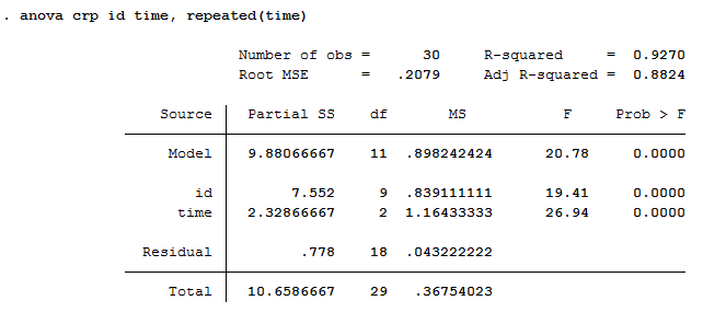
Published with written permission from StataCorp LP.

This table provides all the information we require to report the result of the one-way repeated measures ANOVA if the assumption of sphericity is not violated. To do this, you need to consider the information displayed in the "time" and "Residual" rows. From the "time" row you require the values under the "df" (i.e., "2"), "F" (i.e., "26.94") and "Prob > F" (i.e., "0.0000") columns and the value under the "df" (i.e., "18") column from the "Residual" row. Using this information you can report the result of the one-way repeated measures ANOVA. You can see that the statistical significance of the test (i.e., the "Prob > F" column) is .0000, which we can state as p < .0005. As such, the result is statistically significant.

Alternatively, if the assumption of sphericity was violated, you can choose one of three correction factors so that the result from the one-way repeated measures ANOVA is still valid. These corrections are presented in the table below:

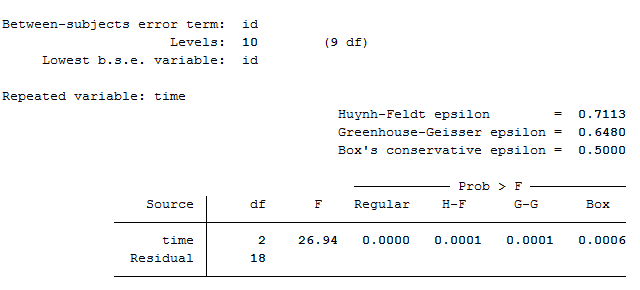
Published with written permission from StataCorp LP.

For example, if we chose to use the Greenhouse-Geisser correction, we would need to consult the statistical significance value (i.e., p-value) under the "G-G" column, which is itself under the "Prob > F" column, in this table rather than the p-value from the first table. You can see that, even with this correction, the result is still statistically significant because p = .0001.

Note: We present the output from the one-way repeated measures ANOVA above. However, since you should have tested your data for the assumptions we explained earlier in the Assumptions section, you will also need to interpret the Stata output that was produced when you tested for them. This includes: (a) the boxplots you used to check if there were any significant outliers; and (b) the output Stata produces for your Shapiro-Wilk test for normality to determine normality. Also, remember that if your data failed any of these assumptions, the output that you get from the one-way repeated measures ANOVA procedure (i.e., the output we discuss above) might no longer be valid, and you will need to interpret the Stata output that is produced when they fail (i.e., this includes different results).

Stata

Reporting the Output of the One-Way Repeated Measures ANOVA

You could report the output of the test above as follows (not including the tests of assumptions or introduction to the analysis):