One-sample t-test using Stata

Introduction

The one-sample t-test is used to determine whether a sample comes from a population with a specific mean. This population mean is not always known, but is sometimes hypothesized.

For example, imagine that you are conducting a study on weight gain and you want to check that the body mass index (BMI) of your 40 participants reflected the national average BMI of approximately 26 (kg/m²). You could use a one-sample t-test to compare the BMI of your 40 participants against the national average. Alternately, imagine that an insurer wanted to check whether taxi drivers were working longer than 80 hours per week, which a new report suggested significantly increased the risk of road accidents. You could use a one-sample t-test to compare the weekly driving hours of a sample of 50 taxi drivers again the 80 hour suggested limit.

In this guide, we show you how to carry out a one-sample t-test using Stata, as well as interpret and report the results from this test. However, before we introduce you to this procedure, you need to understand the different assumptions that your data must meet in order for a one-sample t-test to give you a valid result. We discuss these assumptions next.

Stata

Assumptions

There are four assumptions that underpin the one-sample t-test. If any of these four assumptions are not met, you might not be able to analyze your data using a one-sample t-test because you might not get a valid result. Since assumptions #1 and #2 relate to your study design and choice of variables, they cannot be tested for using Stata. However, you should decide whether your study meets these assumptions before moving on.

• Assumption #1: Your dependent variable should be measured at the continuous level (i.e., it is an interval or ratio variable). Examples of continuous variables include height (measured in feet and inches), temperature (measured in °C), salary (measured in US dollars), revision time (measured in hours), intelligence (measured using IQ score), reaction time (measured in milliseconds), test performance (measured from 0 to 100), sales (measured in number of transactions per month), and so forth. If you are unsure whether your dependent variable is continuous (i.e., measured at the interval or ratio level), see our Types of Variable guide.
• Assumption #2: The data are independent (i.e., not correlated/related), which means that there is no relationship between the observations. This is more of a study design issue than something you can test for, but it is an important assumption of the one-sample t-test.

Fortunately, you can check assumptions #3 and #4 using Stata. When moving on to assumptions #3 and #4, we suggest testing them in this order because it represents an order where, if a violation to the assumption is not correctable, you will no longer be able to use a one-sample t-test. In fact, do not be surprised if your data fails one or more of these assumptions since this is fairly typical when working with real-world data rather than textbook examples, which often only show you how to carry out a one-sample t-test when everything goes well. However, don’t worry because even when your data fails certain assumptions, there is often a solution to overcome this (e.g., transforming your data or using another statistical test instead). Just remember that if you do not check that your data meets these assumptions or you test for them incorrectly, the results you get when running a one-sample t-test might not be valid.

• Assumption #3: There should be no significant outliers. An outlier is simply a case within your data set that does not follow the usual pattern (e.g., in a study of 100 students' IQ scores, where the mean score was 108 with only a small variation between students, one student had a score of 156, which is very unusual, and may even put her in the top 1% of IQ scores globally). The problem with outliers is that they can have a negative effect on the one-sample t-test, reducing the accuracy of your results. Fortunately, when using Stata to run a one-sample t-test on your data, you can easily detect possible outliers.
• Assumption #4: Your dependent variable should be approximately normally distributed. Your data need only be approximately normal for running a one-sample t-test because it is quite "robust" to violations of normality, meaning that this assumption can be a little violated and still provide valid results. You can test for normality using the Shapiro-Wilk test of normality, which is easily tested for using Stata.

In practice, checking for assumptions #3 and #4 will probably take up most of your time when carrying out a one-sample t-test. However, it is not a difficult task, and Stata provides all the tools you need to do this.

In the section, Test Procedure in Stata, we illustrate the Stata procedure required to perform a one-sample t-test assuming that no assumptions have been violated. First, we set out the example we use to explain the one-sample t-test procedure in Stata.

Stata

Example

A lecturer wants to determine how students' test anxiety is affected by the use of a hypnotherapy programme. As such, the lecturer plans to carry out a study where 40 students are split randomly into two equal groups: one group of 20 students who receive the hypnotherapy programme and a second group of 20 students who do not receive the hypnotherapy programme. Then, before all 40 students sit an exam, the lecturer measures their test anxiety. To measure the difference in test anxiety between the two groups of students, the lecturer could then use an independent t-test.

However, before the lecturer carries out this study, he wants to make sure that the 40 students taking part have test anxiety levels that are considered to be 'normal'. Let's imagine that a score of 8.0 is considered to reflect 'normal' test anxiety levels. Lower scores indicate less test anxiety and higher scores indicate greater test anxiety. Therefore, the test anxiety of all 40 participants is measured and a one-sample t-test is used to determine whether this sample is representative of a normal population (i.e., whether the participants' mean test anxiety score is statistically significantly different from 8.0). The test anxiety scores are recorded in the variable, TestAnxiety.

Stata

Setup in Stata

In Stata, we entered the scores for the dependent variable, TestAnxiety, into the Data Editor (Edit) spreadsheet, as shown below:

Published with written permission from StataCorp LP.

Stata

Test Procedure in Stata

In this section, we show you how to analyze your data using a one-sample t-test in Stata when the four assumptions in the previous section, Assumptions, have not been violated. You can carry out a one-sample t-test using code or Stata's graphical user interface (GUI). After you have carried out your analysis, we show you how to interpret your results. First, choose whether you want to use code or Stata's graphical user interface (GUI).

Code

The code to run a one-sample t-test on your data takes the form:

ttest DependentVariable == Hypothesized Value

This code is entered into the box below:

Published with written permission from StataCorp LP.

Using our example where the dependent variable is TestAnxiety and the hypothesized value is 8.0, the required code would be:

ttest TestAnxiety == 8.0

Therefore, enter the code, ttest TestAnxiety == 8.0, and press the "Return/Enter" button on your keyboard.

Published with written permission from StataCorp LP.

You can see the Stata output that will be produced here.

Graphical User Interface (GUI)

The four steps required to run a one-sample t-test in Stata are shown below:

1. Click Statistics > Summaries, tables, and tests > Classical tests of hypotheses > t test (mean-comparison test) on the top menu, as shown below:
   

   Published with written permission from StataCorp LP.

   
   You will be presented with the t tests (mean-comparison tests) dialogue box:
   
   

   Published with written permission from StataCorp LP.

2. Keep the One-sample option in the –t-tests– area, as shown below:
   

   Published with written permission from StataCorp LP.

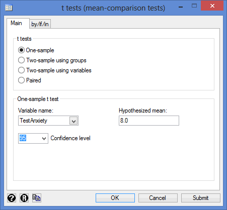
3. Select the dependent variable, TestAnxiety, from within the Variable name: drop-down box, and enter the value of the hypothesized mean, 8.0, in the Hypothesized mean: box. You will end up with a screen similar to the one below:
   

   Published with written permission from StataCorp LP.

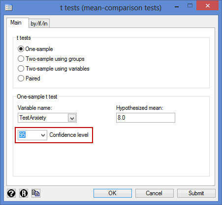
   Note: By default, Stata uses 95% confidence intervals, which equates to declaring statistical significance at the p < .05 level. If you want to change the value of the confidence interval, enter the new value or use the pre-defined values in the Confidence level: box (e.g., a value of 99 would equate to declaring statistical significance at the p < .01 level), highlighted in red below:
   
   

4. Click on the button. The output that Stata produces is shown below.

Stata

Output of the one-sample t-test in Stata

If your data passed assumption #3 (i.e., there were no significant outliers) and assumption #4 (i.e., your dependent variable was approximately normally distributed), which we explained earlier in the Assumptions section, you will only need to interpret the following Stata output for the one-sample t-test:

Published with written permission from StataCorp LP.

This output provides useful descriptive statistics, including the mean (Mean) and 95% confidence interval (CI) (95% Conf. Interval), as well as the actual results from the one-sample t-test. We can see that there is a statistically significant difference between mean test anxiety and the national population value of 8.0 as the p-value in the Pr(|T| > |t|) row (under Ha: mean != 8.0) is less than 0.05 (i.e., based on a 2-tailed significance level).

Note: We present the output from the one-sample t-test above. However, since you should have tested your data for the assumptions we explained earlier in the Assumptions section, you will also need to interpret the Stata output that was produced when you tested for them. This includes: (a) the boxplots you used to check if there were any significant outliers; and (b) the output Stata produces for your Shapiro-Wilk test of normality to determine normality. Also, remember that if your data failed any of these assumptions, the output that you get from the one-sample t-test procedure (i.e., the output we discuss above) might not be valid, and you will need to interpret the Stata output that is produced when they fail (i.e., this includes different results).

Stata

Reporting the output of the one-sample t-test

When you report the output of your one-sample t-test, it is good practice to include:

• A. An introduction to the analysis you carried out.
• B. Information about your sample, including the sample size (Obs).
• C. A statement of whether there was a statistically significant difference between the sample-estimated population mean and the hypothesized population mean, including the mean (Mean) and 95% confidence interval (CI) of the mean (95% Conf. Interval), as well as the observed t-value (t), degrees of freedom (degrees of freedom), and significance level, or more specifically, the 2-tailed p-value (Pr(|T| > |t|)).

Based on the Stata output above, we could report the results of this study as follows: