Paired t-test using Stata

Introduction

The paired t-test, also referred to as the paired-samples t-test or dependent t-test, is used to determine whether the mean of a dependent variable (e.g., weight, anxiety level, salary, reaction time, etc.) is the same in two related groups (e.g., two groups of participants that are measured at two different "time points" or who undergo two different "conditions"). For example, you could use a paired t-test to understand whether there was a difference in managers' salaries before and after undertaking a PhD (i.e., your dependent variable would be "salary", and your two related groups would be the two different "time points"; that is, salaries "before" and "after" undertaking the PhD). Alternately, you could use a paired t-test to understand whether there was a difference in smokers' daily cigarette consumption 6 week after wearing nicotine patches compared with wearing patches that did not contain nicotine, known as a "placebo" (i.e., your dependent variable would be "daily cigarette consumption", and your two related groups would be the two different "conditions" participants were exposed to; that is, cigarette consumption values after wearing "nicotine patches" (the treatment group) compared to after wearing the "placebo" (the control group)). Specifically, you use a paired t-test to determine whether the mean difference between two groups is statistically significantly different to zero.

Note: In Stata 12, you will see that the paired t-test is referred to as the "Mean-comparison test, paired data", whereas in Stata 13, it comes under "t test (mean-comparison tests)".

In this guide, we show you how to carry out a paired t-test using Stata, as well as interpret and report the results from this test. However, before we introduce you to this procedure, you need to understand the different assumptions that your data must meet in order for a paired t-test to give you a valid result. We discuss these assumptions next.

Stata

Assumptions

There are four "assumptions" that underpin the paired t-test. If any of these four assumptions are not met, you cannot analyse your data using a paired t-test because you will not get a valid result. Since assumptions #1 and #2 relate to your study design and choice of variables, they cannot be tested for using Stata. However, you should decide whether your study meets these assumptions before moving on.

• Assumption #1: Your dependent variable should be measured at the interval or ratio level (i.e., they are continuous). Examples of such dependent variables include height (measured in feet and inches), temperature (measured in ^oC), salary (measured in US dollars), revision time (measured in hours), intelligence (measured using IQ score), reaction time (measured in milliseconds), test performance (measured from 0 to 100), sales (measured in number of transactions per month), and so forth. If you are unsure whether your dependent variable is continuous (i.e., measured at the interval or ratio level), see our Types of Variable guide.
• Assumption #2: Your independent variable should consist of two categorical, "related groups" or "matched pairs". "Related groups" indicates that the same subjects are present in both groups. The reason that it is possible to have the same subjects in each group is because each subject has been measured on two occasions on the same dependent variable. For example, you might have measured 50 participants' typing speed using a keyboard (i.e., the dependent variable) before and after they underwent a touch-typing course designed to improve typing speed (i.e., the two "time points" where participants' typing speed was measured – "before" and "after" the touch-typing course – reflect the two "related groups" of the independent variable). Since the same participants were measured at these two time points, the groups are related. It is also common for related groups to reflect to different conditions that all participants undergo (i.e., these conditions are sometimes called interventions, treatments or trials). For example, 30 participants undergo a hypnotherapy programme (condition A) and drug programme (condition B) to determine which is more effective (if any) at treating depression.

Fortunately, you can check assumptions #3 and #4 using Stata. When moving on to assumptions #3 and #4, we suggest testing them in this order because it represents an order where, if a violation of the assumption is not correctable, you will no longer be able to use a paired t-test. In fact, do not be surprised if your data fails one or more of these assumptions since this is fairly typical when working with real-world data rather than textbook examples, which often only show you how to carry out a paired t-test when everything goes well. However, don’t worry because even when your data fails certain assumptions, there is often a solution to overcome this (e.g., transforming your data or using another statistical test instead). Just remember that if you do not check that your data meets these assumptions or you test for them incorrectly, the results you get when running a paired t-test might not be valid.

• Assumption #3: There should be no significant outliers in the differences between the two related groups. An outlier is simply a single data point within your data that does not follow the usual pattern (e.g., in a study of 100 students' IQ scores, where the mean score was 108 with only a small variation between students, one student had a score of 156, which is very unusual, and may even put her in the top 1% of IQ scores globally). The problem with outliers is that they can have a negative effect on the paired t-test, distorting the differences between the two related groups (whether increasing or decreasing the scores on the dependent variable), which reduces the accuracy of your results. In addition, they can affect the statistical significance of the test. Fortunately, when using Stata to run a paired t-test on your data, you can easily detect possible outliers.
• Assumption #4: The distribution of the differences in the dependent variable between the two related groups should be approximately normally distributed. We talk about the paired t-test only requiring approximately normal data because it is quite "robust" to violations of normality, meaning that the assumption can be a little violated and still provide valid results. You can test for normality using the Shapiro-Wilk test of normality, which is easily tested for using Stata.

In practice, checking for assumptions #3 and #4 will probably take up most of your time when carrying out a paired t-test. However, it is not a difficult task, and Stata provides all the tools you need to do this.

In the section, Procedure, we illustrate the Stata procedure required to perform a paired t-test assuming that no assumptions have been violated. First, we set out the example we use to explain the paired t-test procedure in Stata.

Stata

Example

A company researcher wants to test a new formula for a sports drink that has been designed to improve running performance. Instead of the regular "carbohydrate-only" drink that the company produces, this new sports drink contains a "carbohydrate-protein" formula. The researcher would like to know whether this new carbohydrate-protein sports drink leads to a difference in running performance compared to the carbohydrate-only sports drink. Therefore, the dependent variable was "running performance", and the independent variable was "formula", which consisted of two related groups: "carbohydrate-protein" and "carbohydrate-only".

To carry out the experiment, the researcher recruited 20 middle distance runners. All of these participants performed two trials in which they had to run as far as possible for 2 hours on a treadmill. In one of the trials, all 20 participants drank from a bottle containing the carbohydrate-only formula. In the other trial, the same 20 participants drank from a bottle containing the carbohydrate-protein formula. Whilst all participants completed both trials, the order in which they underwent the trials differed, which is known as counterbalancing (i.e., 10 of the 20 participants completed the trial with the carbohydrate-only drink first, and then the trial with the carbohydrate-protein drink second, whilst the other 10 participants started with the carbohydrate-protein trial and then undertook the carbohydrate-only trial). At the end of the two trials, the distance each participant ran (in km) was recorded.

A paired t-test was used to determine whether there was a statistically significant difference in distance run between the two trials (i.e., when using the carbohydrate-protein drink compared to the carbohydrate-only drink).

Stata

Setup in Stata

In Stata, we created two variables: (1) carb, which is the distance run (in km) in two hours for the carbohydrate-only trial; and (2) carb_protein, which is the distance run (in km) in two hours for the carbohydrate-protein trial.

Note: In actual fact, these are not "variables", but rather the two "related groups" of the independent variable, Conditions. However, in Stata, these two related groups will be referred to as variables when you: (a) create them in the first instance; (b) view them in the Data Editor (Edit) spreadsheet, as shown below; and (c) carry out the paired t-test using Stata's dialogue boxes, where Stata refers to them as the "First Variable" and "Second Variable". Therefore, in this guide, we refer to these two related groups as between two variables.

After creating these two variables – carb and carb_protein – we entered the scores for the dependent variable, Distance run, into the two columns of the Data Editor (Edit) spreadsheet (i.e., the distances the participants ran when using the carbohydrate-only drink the left hand column, carb, and the the distances the participants ran when using the carbohydrate-protein drink, carb_protein, the right hand column), as shown below:

Published with written permission from StataCorp LP.

Stata

Test Procedure in Stata

In this section, we show you how to analyse your data using a paired t-test in Stata when the four assumptions in the previous section, Assumptions, have not been violated. You can carry out a paired t-test using code or Stata's graphical user interface (GUI). After you have carried out your analysis, we show you how to interpret your results. First, choose whether you want to use code or Stata's graphical user interface (GUI).

Code

The code to run a paired t-test on your data takes the form:

ttest FirstVariable == SecondVariable

This code is entered into the box below:

Published with written permission from StataCorp LP.

Using our example where the two variables are carb and carb_protein, the required code would be:

ttest carb_protein == carb

Explanation: You need to think carefully about the variables you select as the First variable: and Second variable:. Your study design and aims will determine which variable is most appropriate.

If you have a study design where you are interested in the differences between two "conditions" (see the assumption on related groups if you are unsure what this means), there will often be a control group and an experimental group. In such a case, you will usually subtract the scores on the dependent variable for the control group from your experimental group (i.e., the experimental group minus the control group). The variable that represents the experimental group acts as the First variable: and the variable that represents the control group acts as the Second variable:. Alternately, if your two related groups are two "time points" (e.g., a pre-post study design), you will often subtract the scores on the dependent variable for the first time point from the second time point (e.g., the scores "before" an intervention has taken place from the scores "after" the intervention). In such a case, the second time point acts as the First variable: and the first time point acts as the Second variable:.

In our example, you are interested in whether a new carbohydrate-protein drink (i.e., the experimental group) leads to a difference in performance compared to an existing carbohydrate-only drink (i.e., the control group, since this reflects the status-quo). This way, any positive differences reflect an improvement in the distance run by participants using the carbohydrate-protein drink (carb_protein) compared to the carbohydrate-only drink (carb), and vice-versa for negative differences. Therefore, the carbohydrate-only drink is acting as a control group (carb) and the new carbohydrate-protein drink is acting as the experimental group (carb_protein).

Note 1: By default, Stata uses 95% confidence intervals, which equates to declaring statistical significance at the p < .05 level. However, if you want to change this, you can using the following code:

ttest FirstVariable == SecondVariable, level(ConfidenceIntervalPercentage)

If you wish to change this you can enter any value from 10 to 99.99. For example, entering "99" into this box would result in a 99% confidence interval and equate to declaring statistical significance at the p < .01 level, as shown below:

ttest FirstVariable == SecondVariable, level(99)

Note 2: You need to be precise when entering the code into the box. The code is "case sensitive". For example, if you entered "Carb" where the "C" is uppercase rather than lowercase (i.e., a small "c"), which it should be, you will get an error message like the following:

Note 3: If you're still getting the error message in Note 2: above, it is worth checking the name you gave your two variables in the Data Editor when you set up your file (i.e., see the Data Editor screen above). In the box on the right-hand side of the Data Editor screen, it is the way that you spelt your variables in the section, not the section that you need to enter into the code (see below for our independent variable). This may seem obvious, but it is an error that is sometimes made, resulting in the error in Note 2 above.

Therefore, enter the code, ttest carb_protein == carb, and press the "Return/Enter" button on your keyboard.

Published with written permission from StataCorp LP.

You can see the Stata output that will be produced here.

Graphical User Interface (GUI)

The three steps required to run a paired t-test in Stata 12 – known as a "Mean-comparison test, paired data" in Stata 12 – are shown below. The same procedure requires four steps in Stata 13 and this is shown further down:

Stata

Version 12

1. In Stata 12, click Statistics > Summaries, tables, and tests > Classical tests of hypotheses > Mean-comparison test, paired data on the top menu, as shown below:
   

   Published with written permission from StataCorp LP.

   
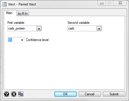
   You will be presented with the ttest - Paired test dialogue box:
   
   

   Published with written permission from StataCorp LP.

2. Select carb_protein from within the First variable: drop-down box, and carb from within the Second variable: drop-down box. For this example, keep the default 95% confidence interval by keeping the 95 value in the Confidence level drop-down box. You will end up with the following screen:
   

   Published with written permission from StataCorp LP.

   Important: Whilst it does not matter which of your two variables you enter into the First variable: and Second variable: dialogue boxes, in order to interpret the Stata output in this guide, we suggest a particular order for selecting these variables, which we discuss in the explanation above. If you follow this explanation, it will be much easier to interpret your results. If you get the order the wrong way around, per se, you have to perform additional calculations using the Stata output that is generated to get your results.

3. Click on the button. This will generate the output.

Stata

Version 13

1. In Stata 13, click Statistics > Summaries, tables, and tests > Classical tests of hypotheses > t test (mean-comparison test) on the top menu, as shown below:
   

   Published with written permission from StataCorp LP.

   
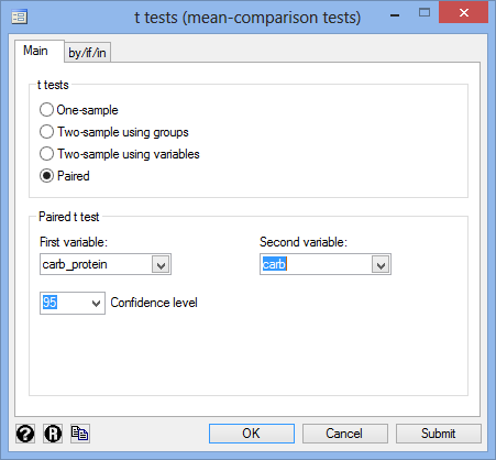
   You will be presented with the t tests (mean-comparison tests) dialogue box:
   
   

   Published with written permission from StataCorp LP.

2. Select the Paired option in the –t-tests– area, as shown below:
   

   Published with written permission from StataCorp LP.

3. In the –Paired t-test– area, select carb_protein from within the First variable: drop-down box, and carb from within the Second variable: drop-down box. For this example, keep the default 95% confidence interval by keeping the 95 value in the Confidence level drop-down box. You will end up with the following screen:
   

   Published with written permission from StataCorp LP.

   Important: Whilst it does not matter which of your two variables you enter into the First variable: and Second variable: dialogue boxes, in order to interpret the Stata output in this guide, we suggest a particular order for selecting these variables, which we discuss in the explanation above. If you follow this explanation, it will be much easier to interpret your results. If you get the order the wrong way around, per se, you have to perform additional calculations using the Stata output that is generated to get your results.

4. Click on the button. The output that Stata produces is shown below.

Stata

Output of the paired t-test in Stata

If your data passed assumption #3 (i.e., there were no significant outliers) and assumption #4 (i.e., the distribution of the differences in your dependent variable between the two related groups was approximately normally distributed), which we explained earlier in the Assumptions section, you will only need to interpret the following Stata output for the paired t-test:

Published with written permission from StataCorp LP.

This output provides useful descriptive statistics for the two groups that you compared, including the mean and standard deviation, as well as actual results from the paired t-test. Looking at the Mean column, you can see that those people who used the nicotine patches had lower cigarette consumptions at the end of the experiment compared to those who received the placebo. You can see that there is a mean difference between the two trials of 0.1355 km (Mean) with a standard deviation of 0.09539 km (Std. Dev.), a standard error of the mean of 0.02133 km (Std. Err.), and 95% confidence intervals of 0.09085 to 0.18015 km (95% Conf. interval). You are presented with an obtained t-value (t) of 6.3524, the degrees of freedom (degrees of freedom), which are 19, and the statistical significance (2-tailed p-value) of the paired t-test (Pr(|T| > |t|) under Ha: mean(diff) != 0), which is 0.0000. As the p-value is less than 0.05 (i.e., p < .05), it can be concluded that there is a statistically significant difference between our two variable scores (carb and carb_protein). In other words, the difference between the two run distances is not equal to zero.

Note: We present the output from the paired t-test above. However, since you should have tested your data for the assumptions we explained earlier in the Assumptions section, you will also need to interpret the Stata output that was produced when you tested for them. This includes: (a) the boxplots you used to check if there were any significant outliers; and (b) the output Stata produces for your Shapiro-Wilk test of normality to determine normality. Also, remember that if your data failed any of these assumptions, the output that you get from the paired t-test procedure (i.e., the output we discuss above) will no longer be relevant, and you will need to interpret the Stata output that is produced when they fail (i.e., this includes different results).

Stata

Reporting the output of the paired t-test

When you report the output of your paired t-test, it is good practice to include: (a) an introduction to the analysis you carried out; (b) information about your sample, including how many participants there were in your sample; (c) the mean and standard deviation for your two related groups; and (d) the observed t-value, 95% confidence intervals, degrees of freedom, and significance level (or more specifically, the 2-tailed p-value). Based on the results above, we could report the results of this study as follows:

In addition to the reporting the results as above, a diagram can be used to visually present your results. For example, you could do this using a bar chart with error bars (e.g., where the errors bars could be the standard deviation, standard error or 95% confidence intervals). This can make it easier for others to understand your results. Furthermore, you are increasingly expected to report "effect sizes" in addition to your paired t-test results. Effect sizes are important because whilst the paired t-test tells you whether differences between group means are "real" (i.e., different in the population), it does not tell you the "size" of the difference. Whilst Stata will not produce these effect sizes for you using the above procedure, there is a procedure in Stata to do so.