Mixed ANOVA using SPSS Statistics

Introduction

A mixed ANOVA compares the mean differences between groups that have been split on two "factors" (also known as independent variables), where one factor is a "within-subjects" factor and the other factor is a "between-subjects" factor. For example, a mixed ANOVA is often used in studies where you have measured a dependent variable (e.g., "back pain" or "salary") over two or more time points or when all subjects have undergone two or more conditions (i.e., where "time" or "conditions" are your "within-subjects" factor), but also when your subjects have been assigned into two or more separate groups (e.g., based on some characteristic, such as subjects' "gender" or "educational level", or when they have undergone different interventions). These groups form your "between-subjects" factor. The primary purpose of a mixed ANOVA is to understand if there is an interaction between these two factors on the dependent variable. Before discussing this further, take a look at the examples below, which illustrate the three more common types of study design where a mixed ANOVA is used:

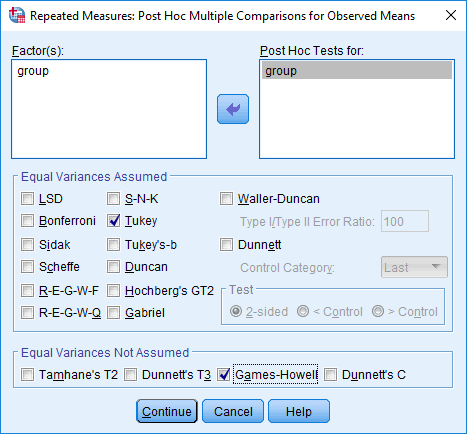
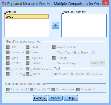
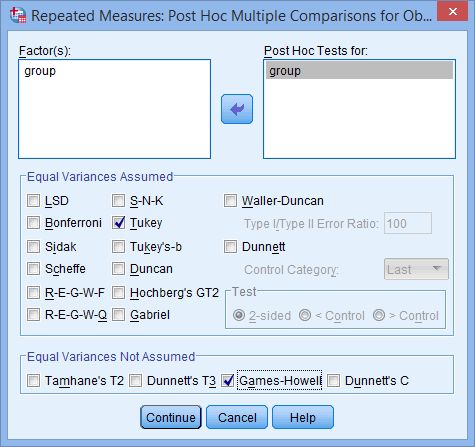
As mentioned above, the primary purpose of a mixed ANOVA is to understand if there is an interaction between your within-subjects factor and between-subjects factor on the dependent variable. Once you have established whether there is a statistically significant interaction, there are a number of different approaches to following up the result. In particular, it is important to realize that the mixed ANOVA is an omnibus test statistic and cannot tell you which specific groups within each factor were significantly different from each other. For example, if one of your factors (e.g., "time") has three groups (e.g., the three groups are your three time points: "time point 1", "time point 2" and "time point 3"), the mixed ANOVA result cannot tell you whether the values on the dependent variable were different for one group (e.g., "Time point 1") compared with another group (e.g., "Time point 2"). It only tells you that at least two of the three groups were different. Since you may have three, four, five or more groups in your study design, as well as two factors, determining which of these groups differ from each other is important. You can do this using post hoc tests, which we discuss later in this guide. In addition, where statistically significant interactions are found, you need to determine whether there are any "simple main effects", and if there are, what these effects are (again, we discuss this later in our guide).

If you are unsure whether a mixed ANOVA is appropriate, you may also want to consider how it differs from a two-way repeated measures ANOVA. Both the mixed ANOVA and two-way repeated measures ANOVA involve two factors, as well as a desire to understand whether there is an interaction between these two factors on the dependent variable. However, the fundamental difference is that a two-way repeated measures ANOVA has two "within-subjects" factors, whereas a mixed ANOVA has only one "within-subjects" factor because the other factor is a "between-subjects" factor. Therefore, in a two-way repeated measures ANOVA, all subjects undergo all conditions (e.g., if the study has two conditions – a control and a treatment – all subjects take part in both the control and the treatment). Therefore, unlike the mixed ANOVA, subjects are not separated into different groups based on some "between-subjects" factor (e.g., a characteristic such as subjects' "gender" or "educational level", or so that they only receive one "condition": either the control or the treatment). Therefore, if you think that the mixed ANOVA is not the test you are looking for, you may want to consider a two-way repeated measures ANOVA. Alternately, if neither of these are appropriate, you can use our Statistical Test Selector, which is part of our enhanced content, to determine which test is appropriate for your study design.

In this "quick start" guide, we show you how to carry out a mixed ANOVA with post hoc tests using SPSS Statistics, as well as the steps you will need to go through to interpret the results from this test. However, before we introduce you to this procedure, you need to understand the different assumptions that your data must meet in order for a mixed ANOVA to give you a valid result. We discuss these assumptions next.

SPSS Statistics

Assumptions

When you choose to analyse your data using a mixed ANOVA, much of the process involves checking to make sure that the data you want to analyse can actually be analysed using a mixed ANOVA. You need to do this because it is only appropriate to use a mixed ANOVA if your data "passes" seven assumptions that are required for a mixed ANOVA to give you a valid result. In practice, checking for these assumptions requires you to use SPSS Statistics to carry out a few more tests, as well as think a little bit more about your data. Whilst it is not a difficult task, it will take up most of your time when carrying out a mixed ANOVA.

Before we introduce you to these seven assumptions, do not be surprised if, when analysing your own data using SPSS Statistics, one or more of these assumptions is violated (i.e., not met). This is not uncommon when working with real-world data rather than textbook examples. However, even when your data fails certain assumptions, there is often a solution to try and overcome this. First, let’s take a look at these seven assumptions:

• Assumption #1: Your dependent variable should be measured at the continuous level (i.e., they are either interval or ratio variables). Examples of continuous variables include revision time (measured in hours), intelligence (measured using IQ score), exam performance (measured from 0 to 100), weight (measured in kg), and so forth. You can learn more about interval and ratio variables in our article: Types of Variable.
• Assumption #2: Your within-subjects factor (i.e., within-subjects independent variable) should consist of at least two categorical, "related groups" or "matched pairs". "Related groups" indicates that the same subjects are present in both groups. The reason that it is possible to have the same subjects in each group is because each subject has been measured on two occasions on the same dependent variable, whether this is at two different "time points" or having undergone two different "conditions". For example, you might have measured 10 individuals' performance in a spelling test (the dependent variable) before and after they underwent a new form of computerized teaching method to improve spelling (i.e., two different "time points"). You would like to know if the computer training improved their spelling performance. The first related group consists of the subjects at the beginning of the experiment, prior to the computerized spelling training, and the second related group consists of the same subjects, but now at the end of the computerized training.
• Assumption #3: Your between-subjects factor (i.e., between-subjects factor independent variable) should each consist of at least two categorical, "independent groups". Example independent variables that meet this criterion include gender (2 groups: male or female), ethnicity (3 groups: Caucasian, African American and Hispanic), physical activity level (4 groups: sedentary, low, moderate and high), profession (5 groups: surgeon, doctor, nurse, dentist, therapist), and so forth.
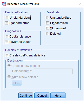
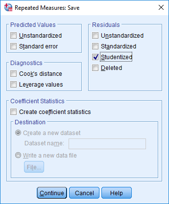
• Assumption #4: There should be no significant outliers in any group of your within-subjects factor or between-subjects factor. Outliers are simply single data points within your data that do not follow the usual pattern (e.g., in a study of 100 students' IQ scores, where the mean score was 108 with only a small variation between students, one student had a score of 156, which is very unusual, and may even put her in the top 1% of IQ scores globally). The problem with outliers is that they can have a negative effect on the mixed ANOVA, distorting the differences between the related groups (whether increasing or decreasing the scores on the dependent variable), which reduces the accuracy of your results. Fortunately, when using SPSS Statistics to run a mixed ANOVA on your data, you can easily detect possible outliers. In our enhanced mixed ANOVA guide, we: (a) show you how to detect outliers using SPSS Statistics, whether you check for outliers in your 'actual data' or using 'studentized residuals'; and (b) discuss some of the options you have in order to deal with outliers.
• Assumption #5: Your dependent variable should be approximately normally distributed for each combination of the groups of your two factors (i.e., your within-subjects factor and between-subjects factor). Whilst this sounds a little tricky, it is easily tested for using SPSS Statistics. Also, when we talk about the mixed only requiring approximately normal data, this is because it is quite "robust" to violations of normality, meaning that assumption can be a little violated and still provide valid results. You can test for normality using, for example, the Shapiro-Wilk test of normality (for 'actual data') or Q-Q Plots (for 'studentized residuals'), both of which are simple procedures in SPSS Statistics. In addition to showing you how to do this in our enhanced mixed ANOVA guide, we also explain what you can do if your data fails this assumption (i.e., if it fails it more than a little bit).
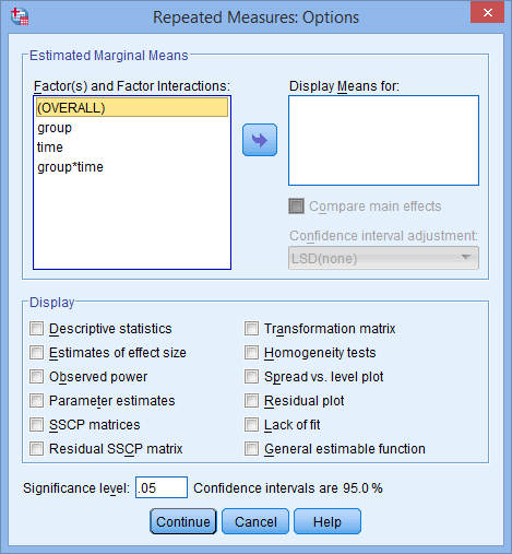
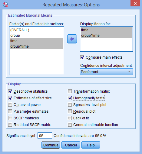
• Assumption #6: There needs to be homogeneity of variances for each combination of the groups of your two factors (i.e., your within-subjects factor and between-subjects factor). Again, whilst this sounds a little tricky, you can easily test this assumption in SPSS Statistics using Levene’s test for homogeneity of variances. In our enhanced mixed ANOVA guide, we (a) show you how to perform Levene’s test for homogeneity of variances in SPSS Statistics, (b) explain some of the things you will need to consider when interpreting your data, and (c) present possible ways to continue with your analysis if your data fails to meet this assumption.
• Assumption #7: Known as sphericity, the variances of the differences between the related groups of the within-subject factor for all groups of the between-subjects factor (i.e., your within-subjects factor and between-subjects factor) must be equal. Fortunately, SPSS Statistics makes it easy to test whether your data has met or failed this assumption. Therefore, in our enhanced mixed ANOVA guide, we (a) show you how to perform Mauchly's Test of Sphericity in SPSS Statistics, (b) explain some of the things you will need to consider when interpreting your data, and (c) present possible ways to continue with your analysis if your data fails to meet this assumption.

You can check assumptions #4, #5, #6 and #7 using SPSS Statistics. Just remember that if you do not run the statistical tests on these assumptions correctly, the results you get when running a mixed ANOVA might not be valid. This is why we dedicate a number of sections in our enhanced guide to help you get this right. You can find out about our enhanced content as a whole on our Features: Overview page, or more specifically, learn how we help with testing assumptions on our Features: Assumptions page.

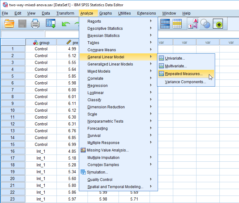
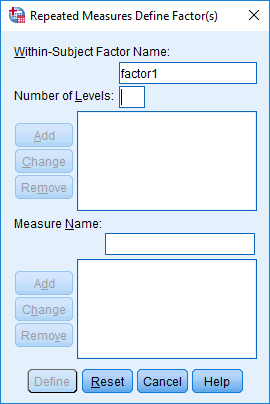
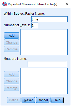
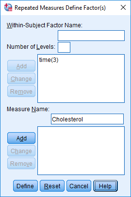
In the section, Procedure, we illustrate the SPSS Statistics procedure that you can use to carry out a mixed ANOVA on your data. First, we introduce the example that is used in this guide.