Pearson Product-Moment Correlation
What does this test do?
The Pearson product-moment correlation coefficient (or Pearson correlation coefficient, for short) is a measure of the strength of a linear association between two variables and is denoted by r. Basically, a Pearson product-moment correlation attempts to draw a line of best fit through the data of two variables, and the Pearson correlation coefficient, r, indicates how far away all these data points are to this line of best fit (i.e., how well the data points fit this new model/line of best fit).
What values can the Pearson correlation coefficient take?
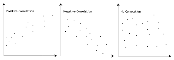
The Pearson correlation coefficient, r, can take a range of values from +1 to -1. A value of 0 indicates that there is no association between the two variables. A value greater than 0 indicates a positive association; that is, as the value of one variable increases, so does the value of the other variable. A value less than 0 indicates a negative association; that is, as the value of one variable increases, the value of the other variable decreases. This is shown in the diagram below:

How can we determine the strength of association based on the Pearson correlation coefficient?
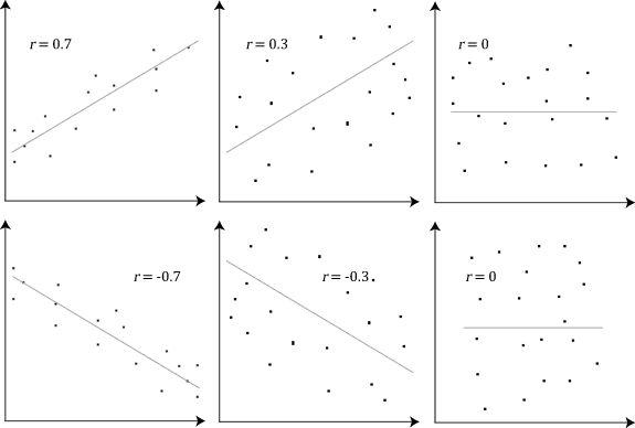
The stronger the association of the two variables, the closer the Pearson correlation coefficient, r, will be to either +1 or -1 depending on whether the relationship is positive or negative, respectively. Achieving a value of +1 or -1 means that all your data points are included on the line of best fit – there are no data points that show any variation away from this line. Values for r between +1 and -1 (for example, r = 0.8 or -0.4) indicate that there is variation around the line of best fit. The closer the value of r to 0 the greater the variation around the line of best fit. Different relationships and their correlation coefficients are shown in the diagram below:
Are there guidelines to interpreting Pearson's correlation coefficient?
Yes, the following guidelines have been proposed:
| |
Coefficient, r |
| Strength of Association |
Positive |
Negative |
| Small |
.1 to .3 |
-0.1 to -0.3 |
| Medium |
.3 to .5 |
-0.3 to -0.5 |
| Large |
.5 to 1.0 |
-0.5 to -1.0 |
Remember that these values are guidelines and whether an association is strong or not will also depend on what you are measuring.
Can you use any type of variable for Pearson's correlation coefficient?
No, the two variables have to be measured on either an interval or ratio scale. However, both variables do not need to be measured on the same scale (e.g., one variable can be ratio and one can be interval). Further information about types of variable can be found in our Types of Variable guide. If you have ordinal data, you will want to use Spearman's rank-order correlation or a Kendall's Tau Correlation instead of the Pearson product-moment correlation.
Do the two variables have to be measured in the same units?
No, the two variables can be measured in entirely different units. For example, you could correlate a person's age with their blood sugar levels. Here, the units are completely different; age is measured in years and blood sugar level measured in mmol/L (a measure of concentration). Indeed, the calculations for Pearson's correlation coefficient were designed such that the units of measurement do not affect the calculation. This allows the correlation coefficient to be comparable and not influenced by the units of the variables used.
What about dependent and independent variables?
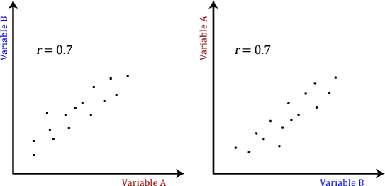
The Pearson product-moment correlation does not take into consideration whether a variable has been classified as a dependent or independent variable. It treats all variables equally. For example, you might want to find out whether basketball performance is correlated to a person's height. You might, therefore, plot a graph of performance against height and calculate the Pearson correlation coefficient. Lets say, for example, that r = .67. That is, as height increases so does basketball performance. This makes sense. However, if we plotted the variables the other way around and wanted to determine whether a person's height was determined by their basketball performance (which makes no sense), we would still get r = .67. This is because the Pearson correlation coefficient makes no account of any theory behind why you chose the two variables to compare. This is illustrated below:
Does the Pearson correlation coefficient indicate the slope of the line?
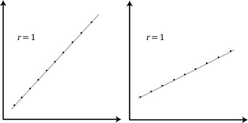
It is important to realize that the Pearson correlation coefficient, r, does not represent the slope of the line of best fit. Therefore, if you get a Pearson correlation coefficient of +1 this does not mean that for every unit increase in one variable there is a unit increase in another. It simply means that there is no variation between the data points and the line of best fit. This is illustrated below:
What assumptions does Pearson's correlation make?
The first and most important step before analysing your data using Pearson’s correlation is to check whether it is appropriate to use this statistical test. After all, Pearson’s correlation will only give you valid/accurate results if your study design and data "pass/meet" seven assumptions that underpin Pearson’s correlation.
In many cases, Pearson’s correlation will be the incorrect statistical test to use because your data "violates/does not meet" one or more of these assumptions. This is not uncommon when working with real-world data, which is often "messy", as opposed to textbook examples. However, there is often a solution, whether this involves using a different statistical test, or making adjustments to your data so that you can continue to use Pearson’s correlation.
We briefly set out the seven assumptions below, three of which relate to your study design and how you measured your variables (i.e., Assumptions #1, #2 and #3 below), and four which relate to the characteristics of your data (i.e., Assumptions #4, #5, #6 and #7 below):
Note: We list seven assumptions below, but there is disagreement in the statistics literature whether the term "assumptions" should be used to describe all of these (e.g., see Nunnally, 1978). We highlight this point for transparency. However, we use the word "assumptions" to stress their importance and to indicate that they should be examined closely when using a Pearson’s correlation if you want accurate/valid results. We also use the word "assumptions" to indicate that where some of these are not met, Pearson’s correlation will no longer be the correct statistical test to analyse your data.
Since assumptions #1, #2 and #3 relate to your study design and how you measured your variables, if any of these three assumptions are not met (i.e., if any of these assumptions do not fit with your research), Pearson’s correlation is the incorrect statistical test to analyse your data. It is likely that there will be other statistical tests you can use instead, but Pearson’s correlation is not the correct test.
After checking if your study design and variables meet assumptions #1, #2 and #3, you should now check if your data also meets assumptions #4, #5, #6 and #7 below. When checking if your data meets these four assumptions, do not be surprised if this process takes up the majority of the time you dedicate to carrying out your analysis. As we mentioned above, it is not uncommon for one or more of these assumptions to be violated (i.e., not met) when working with real-world data rather than textbook examples. However, with the right guidance this does not need to be a difficult process and there are often other statistical analysis techniques that you can carry out that will allow you to continue with your analysis.
Note: If your two continuous, paired variables (i.e., Assumptions #1 and 2) follow a bivariate normal distribution, there will be linearity, univariate normality and homoscedasticity (i.e., Assumptions #4, #5 and #6 below; e.g., Lindeman et al., 1980). Unfortunately, the assumption of bivariate normality is very difficult to test, which is why we focus on linearity and univariate normality instead. Homoscedasticity is also difficult to test, but we include this so that you know why it is important. We include outliers at the end (i.e., Assumption #7) because they cannot only lead to violations of the linearity and univariate normality assumptions, but they also have a large impact on the value of Pearson’s correlation coefficient, r (e.g., Wilcox, 2012).
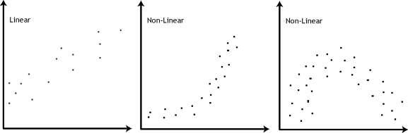
- Assumption #4: There should be a linear relationship between your two continuous variables. To test to see whether your two variables form a linear relationship you simply need to plot them on a graph (a scatterplot, for example) and visually inspect the graph's shape. In the diagram below, you will find a few different examples of a linear relationship and some non-linear relationships. It is not appropriate to analyse a non-linear relationship using a Pearson product-moment correlation.
Note: Pearson's correlation coefficient is a measure of the strength of a linear association between two variables. Put another way, it determines whether there is a linear component of association between two continuous variables. As such, linearity is not strictly an "assumption" of Pearson's correlation. However, you would not normally want to use Pearson's correlation to determine the strength and direction of a linear relationship when you already know the relationship between your two variables is not linear. Instead, the relationship between your two variables might be better described by another statistical measure (Cohen, 2013). For this reason, it is not uncommon to view the relationship between your two variables in a scatterplot to see if running a Pearson's correlation is the best choice as a measure of association or whether another measure would be better.
- Assumption #5: Theoretically, both continuous variables should follow a bivariate normal distribution, although in practice it is frequently accepted that simply having univariate normality in both variables is sufficient (i.e., each variable is normally distributed). When one or both variables is not normally distributed, there is disagreement about whether Pearson’s correlation will still provide a valid result (i.e., there is disagreement about whether Pearson’s correlation is "robust" to violations of univariate normality). If you do not accept the arguments that Pearson’s correlation is robust to a lack of univariate normality in one or both variables, there are more robust methods that can be considered instead (e.g., see Shevlyakov and Oja, 2016).
Note: The disagreements about the robustness of Pearson’s correlation are based on additional assumptions that are made to justify robustness under non-normality and whether these additional assumptions are likely to be true in practice. For further reading on this issue, see, for example, Edgell and Noon (1984) and Hogg and Craig (2014).
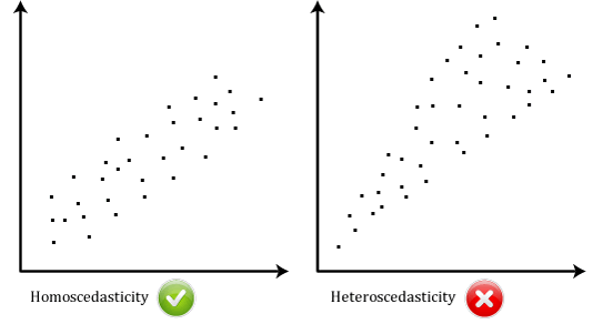
- Assumption #6: There should be homoscedasticity, which means that the variances along the line of best fit remain similar as you move along the line. If the variances are not similar, there is heteroscedasticity. Homoscedasticity is most easily demonstrated diagrammatically, as shown below:
Unfortunately, it is difficult to test for homoscedasticity in a Pearson’s correlation, but where you believe that this may be a problem, there are methods that may be able to help (e.g., see Wilcox, 2012, for some advanced methods).
- Assumption #7: There should be no univariate or multivariate outliers. An outlier is an observation within your sample that does not follow a similar pattern to the rest of your data. Remember that in a Pearson’s correlation, each case (e.g., each participant) will have two values/observations (e.g., a value for revision time and an exam score). You need to consider outliers that are unusual only on one variable, known as "univariate outliers", as well as those that are an unusual "combination" of both variables, known as "multivariate outliers".
Consider the example of revision time and exam score. If all university students scored between 45% and 95% in their exam except for one who scored a very low 5% in their exam, this individual would be a "univariate" outlier. That is, they have an unusual score for this specific variable irrespective of the values of the other variable, revision time. A multivariate outlier is an outlier that "bucks the trend" of the data. A multivariate outlier need not be a univariate outlier. Let’s assume that time spent revising is positively correlated with exam score (i.e., the more a student studied, the higher their exam mark). If a university student did almost no studying, but "aced" the exam, they would be a multivariate outlier. Conversely, if someone revised more than most, but scored badly, they might be a multivariate outlier.
For example, imagine that one of the 100 university students’ scored 5 out of 100 in their exam. An exam score of 5 of our 100 would be unusual compared to the other 99 students, whereas the other 99 students all scored somewhere between 45 and 95 out of 100 in their exam. Therefore, this would be a "univariate outlier". In other words, the student has an unusual score for this specific variable, "exam score", irrespective of what values they had on the other variable, "revision time". Alternatively, a "multivariate outlier" is an outlier that "bucks the trend" of the data. Also, a multivariate outlier need not be a univariate outlier. Therefore, let’s assume that the amount of time a student spends revising is positively correlated with their exam score (i.e., the more a student studies, the higher their exam score). If a student did almost no revision whatsoever, but achieved the highest exam score, they might be a multivariate outlier. Conversely, if another student revised more than most, but scored badly, they might also be a multivariate outlier.
Note: Outliers are not necessarily "bad", but due to the effect they have on the Pearson correlation coefficient, r, discussed on the next page, they need to be taken into account.
You can check whether your data meets assumptions #4, #5 and #7 using a number of statistics packages (to learn more, see our guides for: SPSS Statistics, Stata and Minitab). If any of these seven assumptions are violated (i.e., not met), there are often other statistical analysis techniques that you can carry out that will allow you to continue with your analysis (e.g., see Shevlyakov and Oja, 2016).
On the next page we discuss other characteristics of Pearson's correlation that you should consider.