Linear regression analysis using Stata

Introduction

Linear regression, also known as simple linear regression or bivariate linear regression, is used when we want to predict the value of a dependent variable based on the value of an independent variable. For example, you could use linear regression to understand whether exam performance can be predicted based on revision time (i.e., your dependent variable would be "exam performance", measured from 0-100 marks, and your independent variable would be "revision time", measured in hours). Alternately, you could use linear regression to understand whether cigarette consumption can be predicted based on smoking duration (i.e., your dependent variable would be "cigarette consumption", measured in terms of the number of cigarettes consumed daily, and your independent variable would be "smoking duration", measured in days). If you have two or more independent variables, rather than just one, you need to use multiple regression. Alternatively, if you just wish to establish whether a linear relationship exists, you could use Pearson's correlation.

Note: The dependent variable is also referred to as the outcome, target or criterion variable, whilst the independent variable is also referred to as the predictor, explanatory or regressor variable. Ultimately, whichever term you use, it is best to be consistent. We will refer to these as dependent and independent variables throughout this guide.

In this guide, we show you how to carry out linear regression using Stata, as well as interpret and report the results from this test. However, before we introduce you to this procedure, you need to understand the different assumptions that your data must meet in order for linear regression to give you a valid result. We discuss these assumptions next.

Stata

Assumptions

There are seven "assumptions" that underpin linear regression. If any of these seven assumptions are not met, you cannot analyse your data using linear because you will not get a valid result. Since assumptions #1 and #2 relate to your choice of variables, they cannot be tested for using Stata. However, you should decide whether your study meets these assumptions before moving on.

• Assumption #1: Your dependent variable should be measured at the continuous level. Examples of such continuous variables include height (measured in feet and inches), temperature (measured in ^oC), salary (measured in US dollars), revision time (measured in hours), intelligence (measured using IQ score), reaction time (measured in milliseconds), test performance (measured from 0 to 100), sales (measured in number of transactions per month), and so forth. If you are unsure whether your dependent variable is continuous (i.e., measured at the interval or ratio level), see our Types of Variable guide.
• Assumption #2: Your independent variable should be measured at the continuous or categorical level. However, if you have a categorical independent variable, it is more common to use an independent t-test (for 2 groups) or one-way ANOVA (for 3 groups or more). In case you are unsure, examples of categorical variables include gender (e.g., 2 groups: male and female), ethnicity (e.g., 3 groups: Caucasian, African American and Hispanic), physical activity level (e.g., 4 groups: sedentary, low, moderate and high), and profession (e.g., 5 groups: surgeon, doctor, nurse, dentist, therapist). In this guide, we show you the linear regression procedure and Stata output when both your dependent and independent variables were measured on a continuous level.

Fortunately, you can check assumptions #3, #4, #5, #6 and #7 using Stata. When moving on to assumptions #3, #4, #5, #6 and #7, we suggest testing them in this order because it represents an order where, if a violation to the assumption is not correctable, you will no longer be able to use linear regression. In fact, do not be surprised if your data fails one or more of these assumptions since this is fairly typical when working with real-world data rather than textbook examples, which often only show you how to carry out linear regression when everything goes well. However, don’t worry because even when your data fails certain assumptions, there is often a solution to overcome this (e.g., transforming your data or using another statistical test instead). Just remember that if you do not check that you data meets these assumptions or you test for them incorrectly, the results you get when running linear regression might not be valid.

• Assumption #3: There needs to be a linear relationship between the dependent and independent variables. Whilst there are a number of ways to check whether a linear relationship exists between your two variables, we suggest creating a scatterplot using Stata, where you can plot the dependent variable against your independent variable. You can then visually inspect the scatterplot to check for linearity. Your scatterplot may look something like one of the following:
  
  
  
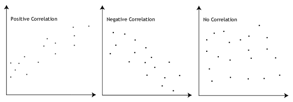
  If the relationship displayed in your scatterplot is not linear, you will have to either run a non-linear regression analysis or "transform" your data, which you can do using Stata.
• Assumption #4: There should be no significant outliers. Outliers are simply single data points within your data that do not follow the usual pattern (e.g., in a study of 100 students' IQ scores, where the mean score was 108 with only a small variation between students, one student had a score of 156, which is very unusual, and may even put her in the top 1% of IQ scores globally). The following scatterplots highlight the potential impact of outliers:
  
  
  
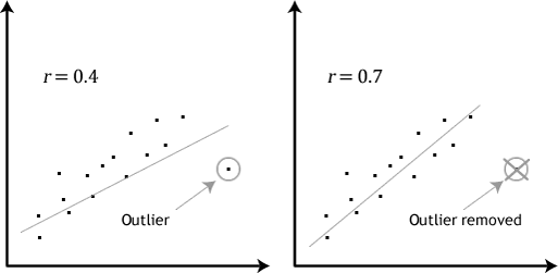
  The problem with outliers is that they can have a negative effect on the regression equation that is used to predict the value of the dependent variable based on the independent variable. This will change the output that Stata produces and reduce the predictive accuracy of your results. Fortunately, you can use Stata to carry out casewise diagnostics to help you detect possible outliers.
• Assumption #5: You should have independence of observations, which you can easily check using the Durbin-Watson statistic, which is a simple test to run using Stata.
• Assumption #6: Your data needs to show homoscedasticity, which is where the variances along the line of best fit remain similar as you move along the line. The two scatterplots below provide simple examples of data that meets this assumption and one that fails the assumption:
  
  
  
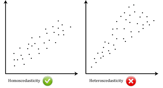
  When you analyse your own data, you will be lucky if your scatterplot looks like either of the two above. Whilst these help to illustrate the differences in data that meets or violates the assumption of homoscedasticity, real-world data is often a lot more messy. You can check whether your data showed homoscedasticity by plotting the regression standardized residuals against the regression standardized predicted value.
• Assumption #7: Finally, you need to check that the residuals (errors) of the regression line are approximately normally distributed. Two common methods to check this assumption include using either a histogram (with a superimposed normal curve) or a Normal P-P Plot.

In practice, checking for assumptions #3, #4, #5, #6 and #7 will probably take up most of your time when carrying out linear regression. However, it is not a difficult task, and Stata provides all the tools you need to do this.

In the section, Procedure, we illustrate the Stata procedure required to perform linear regression assuming that no assumptions have been violated. First, we set out the example we use to explain the linear regression procedure in Stata.

Stata

Example

Studies show that exercising can help prevent heart disease. Within reasonable limits, the more you exercise, the less risk you have of suffering from heart disease. One way in which exercise reduces your risk of suffering from heart disease is by reducing a fat in your blood, called cholesterol. The more you exercise, the lower your cholesterol concentration. Furthermore, it has recently been shown that the amount of time you spend watching TV – an indicator of a sedentary lifestyle – might be a good predictor of heart disease (i.e., that is, the more TV you watch, the greater your risk of heart disease).

Therefore, a researcher decided to determine if cholesterol concentration was related to time spent watching TV in otherwise healthy 45 to 65 year old men (an at-risk category of people). For example, as people spent more time watching TV, did their cholesterol concentration also increase (a positive relationship); or did the opposite happen? The researcher also wanted to know the proportion of cholesterol concentration that time spent watching TV could explain, as well as being able to predict cholesterol concentration. The researcher could then determine whether, for example, people that spent eight hours spent watching TV per day had dangerously high levels of cholesterol concentration compared to people watching just two hours of TV.

To carry out the analysis, the researcher recruited 100 healthy male participants between the ages of 45 and 65 years old. The amount of time spent watching TV (i.e., the independent variable, time_tv) and cholesterol concentration (i.e., the dependent variable, cholesterol) were recorded for all 100 participants. Expressed in variable terms, the researcher wanted to regress cholesterol on time_tv.

Note: The example and data used for this guide are fictitious. We have just created them for the purposes of this guide.

Stata

Setup in Stata

In Stata, we created two variables: (1) time_tv, which is the average daily time spent watching TV in minutes (i.e., the independent variable); and (2) cholesterol, which is the cholesterol concentration in mmol/L (i.e., the dependent variable).

Note: It does not matter whether you create the dependent or independent variable first.

After creating these two variables – time_tv and cholesterol – we entered the scores for each into the two columns of the Data Editor (Edit) spreadsheet (i.e., the time in hours that the participants watched TV in the left-hand column (i.e., time_tv, the independent variable), and participants' cholesterol concentration in mmol/L in the right-hand column (i.e., cholesterol, the dependent variable), as shown below:

Published with written permission from StataCorp LP.

Stata

Test Procedure in Stata

In this section, we show you how to analyse your data using linear regression in Stata when the six assumptions in the previous section, Assumptions, have not been violated. You can carry out linear regression using code or Stata's graphical user interface (GUI). After you have carried out your analysis, we show you how to interpret your results. First, choose whether you want to use code or Stata's graphical user interface (GUI).

Code

The code to carry out linear regression on your data takes the form:

regress DependentVariable IndependentVariable

This code is entered into the box below:

Published with written permission from StataCorp LP.

Using our example where the dependent variable is cholesterol and the independent variable is time_tv, the required code would be:

regress cholesterol time_tv

Note 1: You need to be precise when entering the code into the box. The code is "case sensitive". For example, if you entered "Cholesterol" where the "C" is uppercase rather than lowercase (i.e., a small "c"), which it should be, you will get an error message like the following:

Note 2: If you're still getting the error message in Note 2: above, it is worth checking the name you gave your two variables in the Data Editor when you set up your file (i.e., see the Data Editor screen above). In the box on the right-hand side of the Data Editor screen, it is the way that you spelt your variables in the section, not the section that you need to enter into the code (see below for our dependent variable). This may seem obvious, but it is an error that is sometimes made, resulting in the error in Note 2 above.

Therefore, enter the code, regress cholesterol time_tv, and press the "Return/Enter" button on your keyboard.

Published with written permission from StataCorp LP.

You can see the Stata output that will be produced here.

Graphical User Interface (GUI)

The three steps required to carry out linear regression in Stata 12 and 13 are shown below:

1. Click Statistics > Linear models and related > Linear regression on the main menu, as shown below:
   

   Published with written permission from StataCorp LP.

   
   You will be presented with the Regress – Linear regression dialogue box:
   
   

   Published with written permission from StataCorp LP.

2. Select cholesterol from within the Dependent variable: drop-down box, and time_tv from within the Independent variables: drop-down box. You will end up with the following screen:
   

   Published with written permission from StataCorp LP.

3. Click on the button. This will generate the output.

Stata

Output of linear regression analysis in Stata

If your data passed assumption #3 (i.e., there was a linear relationship between your two variables), #4 (i.e., there were no significant outliers), assumption #5 (i.e., you had independence of observations), assumption #6 (i.e., your data showed homoscedasticity) and assumption #7 (i.e., the residuals (errors) were approximately normally distributed), which we explained earlier in the Assumptions section, you will only need to interpret the following linear regression output in Stata:

Published with written permission from StataCorp LP.

The output consists of four important pieces of information: (a) the R² value ("R-squared" row) represents the proportion of variance in the dependent variable that can be explained by our independent variable (technically it is the proportion of variation accounted for by the regression model above and beyond the mean model). However, R² is based on the sample and is a positively biased estimate of the proportion of the variance of the dependent variable accounted for by the regression model (i.e., it is too large); (b) an adjusted R² value ("Adj R-squared" row), which corrects positive bias to provide a value that would be expected in the population; (c) the F value, degrees of freedom ("F( 1, 98)") and statistical significance of the regression model ("Prob > F" row); and (d) the coefficients for the constant and independent variable ("Coef." column), which is the information you need to predict the dependent variable, cholesterol, using the independent variable, time_tv.

In this example, R² = 0.151. Adjusted R² = 0.143 (to 3 d.p.), which means that the independent variable, time_tv, explains 14.3% of the variability of the dependent variable, cholesterol, in the population. Adjusted R² is also an estimate of the effect size, which at 0.143 (14.3%), is indicative of a medium effect size, according to Cohen's (1988) classification. However, normally it is R² not the adjusted R² that is reported in results. In this example, the regression model is statistically significant, F(1, 98) = 17.47, p = .0001. This indicates that, overall, the model applied can statistically significantly predict the dependent variable, cholesterol.

Note: We present the output from the linear regression analysis above. However, since you should have tested your data for the assumptions we explained earlier in the Assumptions section, you will also need to interpret the Stata output that was produced when you tested for these assumptions. This includes: (a) the scatterplots you used to check if there was a linear relationship between your two variables (i.e., Assumption #3); (b) casewise diagnostics to check there were no significant outliers (i.e., Assumption #4); (c) the output from the Durbin-Watson statistic to check for independence of observations (i.e., Assumption #5); (d) a scatterplot of the regression standardized residuals against the regression standardized predicted value to determine whether your data showed homoscedasticity (i.e., Assumption #6); and a histogram (with superimposed normal curve) and Normal P-P Plot to check whether the residuals (errors) were approximately normally distributed (i.e., Assumption #7). Also, remember that if your data failed any of these assumptions, the output that you get from the linear regression procedure (i.e., the output we discuss above) will no longer be relevant, and you may have to carry out an different statistical test to analyse your data.

Stata

Reporting the output of linear regression analysis

When you report the output of your linear regression, it is good practice to include: (a) an introduction to the analysis you carried out; (b) information about your sample, including any missing values; (c) the observed F-value, degrees of freedom and significance level (i.e., the p-value); (d) the percentage of the variability in the dependent variable explained by the independent variable (i.e., your Adjusted R² ); and (e) the regression equation for your model. Based on the results above, we could report the results of this study as follows:

In addition to the reporting the results as above, a diagram can be used to visually present your results. For example, you could do this using a scatterplot with confidence and prediction intervals (although it is not very common to add the last). This can make it easier for others to understand your results. Furthermore, you can use your linear regression equation to make predictions about the value of the dependent variable based on different values of the independent variable. Whilst Stata does not produce these values as part of the linear regression procedure above, there is a procedure in Stata that you can use to do so.