Multiple Regression Analysis using Stata

Introduction

Multiple regression (an extension of simple linear regression) is used to predict the value of a dependent variable (also known as an outcome variable) based on the value of two or more independent variables (also known as predictor variables). For example, you could use multiple regression to determine if exam anxiety can be predicted based on coursework mark, revision time, lecture attendance and IQ score (i.e., the dependent variable would be "exam anxiety", and the four independent variables would be "coursework mark", "revision time", "lecture attendance" and "IQ score"). Alternately, you could use multiple regression to determine if income can be predicted based on age, gender and educational level (i.e., the dependent variable would be "income", and the three independent variables would be "age", "gender" and "educational level"). If you have a dichotomous dependent variable you can use a binomial logistic regression.

Multiple regression also allows you to determine the overall fit (variance explained) of the model and the relative contribution of each of the independent variables to the total variance explained. For example, you might want to know how much of the variation in exam anxiety can be explained by coursework mark, revision time, lecture attendance and IQ score "as a whole", but also the "relative contribution" of each independent variable in explaining the variance.

This "quick start" guide shows you how to carry out multiple regression using Stata, as well as how to interpret and report the results from this test. However, before we introduce you to this procedure, you need to understand the different assumptions that your data must meet in order for multiple regression to give you a valid result. We discuss these assumptions next.

Stata

Assumptions

There are eight "assumptions" that underpin multiple regression. If any of these eight assumptions are not met, you cannot analyze your data using multiple regression because you will not get a valid result. Since assumptions #1 and #2 relate to your choice of variables, they cannot be tested for using Stata. However, you should decide whether your study meets these assumptions before moving on.

• Assumption #1: Your dependent variable should be measured at the continuous level. Examples of such continuous variables include height (measured in feet and inches), temperature (measured in °C), salary (measured in US dollars), revision time (measured in hours), intelligence (measured using IQ score), reaction time (measured in milliseconds), test performance (measured from 0 to 100), sales (measured in number of transactions per month), and so forth. If you are unsure whether your dependent variable is continuous (i.e., measured at the interval or ratio level), see our Types of Variable guide.
• Assumption #2: You have two or more independent variables, which should be measured at the continuous or categorical level. For examples of continuous variables, see the bullet above. Examples of categorical variables include gender (e.g., 2 groups: male and female), ethnicity (e.g., 3 groups: Caucasian, African American and Hispanic), physical activity level (e.g., 4 groups: sedentary, low, moderate and high), profession (e.g., 5 groups: surgeon, doctor, nurse, dentist, therapist), and so forth. In this guide, we show you the multiple regression procedure because we have a mix of continuous and categorical independent variables.

  Note: If you only have categorical independent variables (i.e., no continuous independent variables), it is more common to approach the analysis from the perspective of a two-way ANOVA (for two categorical independent variables) or factorial ANOVA (for three or more categorical independent variables) instead of multiple regression.

Fortunately, you can check assumptions #3, #4, #5, #6, #7 and #8 using Stata. When moving on to assumptions #3, #4, #5, #6, #7 and #8, we suggest testing them in this order because it represents an order where, if a violation to the assumption is not correctable, you will no longer be able to use multiple regression. In fact, do not be surprised if your data fails one or more of these assumptions since this is fairly typical when working with real-world data rather than textbook examples, which often only show you how to carry out linear regression when everything goes well. However, don’t worry because even when your data fails certain assumptions, there is often a solution to overcome this (e.g., transforming your data or using another statistical test instead). Just remember that if you do not check that you data meets these assumptions or you test for them correctly, the results you get when running multiple regression might not be valid.

• Assumption #3: You should have independence of observations (i.e., independence of residuals), which you can check in Stata using the Durbin-Watson statistic.
• Assumption #4: There needs to be a linear relationship between (a) the dependent variable and each of your independent variables, and (b) the dependent variable and the independent variables collectively. You can check for linearity in Stata using scatterplots and partial regression plots.
• Assumption #5: Your data needs to show homoscedasticity, which is where the variances along the line of best fit remain similar as you move along the line. You can check for homoscedasticity in Stata by plotting the studentized residuals against the unstandardized predicted values.
• Assumption #6: Your data must not show multicollinearity, which occurs when you have two or more independent variables that are highly correlated with each other. You can check this assumption in Stata through an inspection of correlation coefficients and Tolerance/VIF values.
• Assumption #7: There should be no significant outliers, high leverage points or highly influential points, which represent observations in your data set that are in some way unusual. These can have a very negative effect on the regression equation that is used to predict the value of the dependent variable based on the independent variables. You can check for outliers, leverage points and influential points using Stata.
• Assumption #8: The residuals (errors) should be approximately normally distributed, which you can check in Stata using a histogram (with a superimposed normal curve) and Normal P-P Plot, or a Normal Q-Q Plot of the studentized residuals.

In practice, checking for assumptions #3, #4, #5, #6, #7 and #8 will probably take up most of your time when carrying out multiple regression. However, it is not a difficult task, and Stata provides all the tools you need to do this.

In the section, Test Procedure in Stata, we illustrate the Stata procedure required to perform multiple regression assuming that no assumptions have been violated. First, we set out the example we use to explain the multiple regression procedure in Stata.

Stata

Example

A health researcher wants to be able to predict "VO₂max", an indicator of fitness and health. Normally, to perform this procedure requires expensive laboratory equipment, as well as requiring individuals to exercise to their maximum (i.e., until they can no longer continue exercising due to physical exhaustion). This can put off individuals who are not very active/fit and those who might be at higher risk of ill health (e.g., older unfit subjects). For these reasons, it has been desirable to find a way of predicting an individual's VO₂max based on attributes that can be measured more easily and cheaply. To this end, a researcher recruited 100 participants to perform a maximum VO₂max test, but also recorded their "age", "weight", "heart rate" and "gender". Heart rate is the average of the last 5 minutes of a 20 minute, much easier, lower workload cycling test. The researcher's goal is to be able to predict VO₂max based on these four attributes: age, weight, heart rate and gender.

Note: The example and data used for this guide are fictitious. We have just created them for the purposes of this guide.

Stata

Setup in Stata

In Stata, we created five variables: (1) VO₂max, which is the maximal aerobic capacity (i.e., the dependent variable); and (2) age, which is the participant's age; (3) weight, which is the participant's weight (technically, it is their 'mass'); (4) heart_rate, which is the participant's heart rate; and (5) gender, which is the participant's gender (i.e., the independent variables).

After creating these five variables, we entered the scores for each into the five columns of the Data Editor (Edit) spreadsheet, as shown below:

Published with written permission from StataCorp LP.

Stata

Test Procedure in Stata

In this section, we show you how to analyze your data using multiple regression in Stata when the eight assumptions in the previous section, Assumptions, have not been violated. You can carry out multiple regression using code or Stata's graphical user interface (GUI). After you have carried out your analysis, we show you how to interpret your results. First, choose whether you want to use code or Stata's graphical user interface (GUI).

Code

The code to carry out multiple regression on your data takes the form:

regress DependentVariable IndependentVariable#1 IndependentVariable#2 IndependentVariable#3 IndependentVariable#4

This code is entered into the box below:

Using our example where the dependent variable is VO2max and the four independent variables are age, weight, heart_rate and gender, the required code would be:

regress VO2max age weight heart_rate i.gender

Note: You'll see from the code above that continuous independent variables are simply entered "as is", whilst categorical independent variables have the prefix "i" (e.g., age for age, since this is a continuous independent variable, but i.gender for gender, since this is a categorical independent variable).

Therefore, enter the code, regress VO2max age weight heart_rate i.gender, and press the "Return/Enter" button on your keyboard.

You can see the Stata output that will be produced here.

Graphical User Interface (GUI)

The seven steps required to carry out multiple regression in Stata are shown below:

1. Click Statistics > Linear models and related > Linear regression on the main menu, as shown below:
   

   Published with written permission from StataCorp LP.

   Note: Don't worry that you're selecting Statistics > Linear models and related > Linear regression on the main menu, or that the dialogue boxes in the steps that follow have the title, Linear regression. You have not made a mistake. You are in the correct place to carry out the multiple regression procedure. This is just the title that Stata gives, even when running a multiple regression procedure.

2. You will be presented with the regress - Linear regression dialogue box, as shown below:
   

   Published with written permission from StataCorp LP.

3. Select the dependent variable, VO2max, from the Dependent variable: box and select the continuous independent variables, age, weight and heart_rate from the Independent variables: box, using the drop-down button, as shown below:
   

   Published with written permission from StataCorp LP.

4. Select the categorical independent variable, gender, from the Independent variables: box, by first clicking on the button. This will present you with the following dialogue box where your continuous independent variables (age, weight and heart_rate) will have already been entered into the Varlist: box:
   

   Published with written permission from StataCorp LP.

5. Leave Factor variable selected in the –Type of variable– area. Next, in the –Add factor variable– area, leave selected in the Specification: box. Now, select gender in the Variables box using the drop-down button, and then select "Default" in the Base box. Finally, click on the button. You will be presented with the following dialogue box where the categorical independent variable, i.gender, has been entered into the Varlist: box:
   

   Published with written permission from StataCorp LP.

6. Click on the button. You will be returned to the regress - Linear regression dialogue box, but with the categorical independent variable, i.gender, now entered into the Independent variables: box, as shown below:
   

   Published with written permission from StataCorp LP.

7. Click on the button. This will generate the output.

Stata

Interpreting and Reporting the Stata Output of Multiple Regression Analysis

Stata will generate a single piece of output for a multiple regression analysis based on the selections made above, assuming that the eight assumptions required for multiple regression have been met.

Determining how well the model fits

The R² and adjusted R² can be used to determine how well a regression model fits the data:

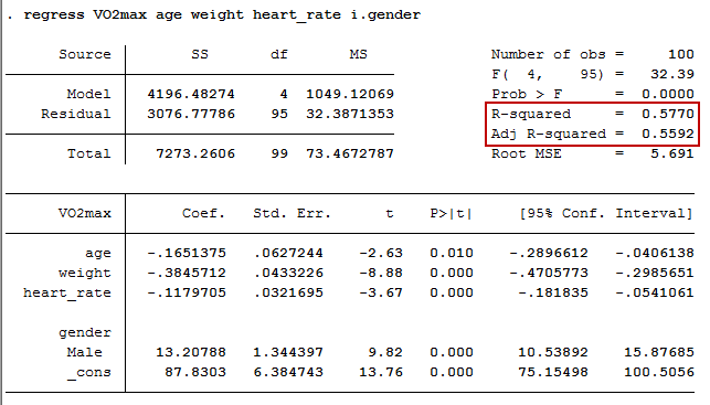
The "R-squared" row represents the R² value (also called the coefficient of determination), which is the proportion of variance in the dependent variable that can be explained by the independent variables (technically, it is the proportion of variation accounted for by the regression model above and beyond the mean model). You can see from our value of 0.577 that our independent variables explain 57.7% of the variability of our dependent variable, VO₂max. However, you also need to be able to interpret "Adj R-squared" (adj. R²) to accurately report your data.

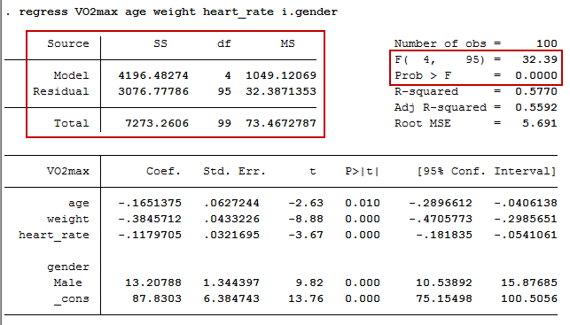
Statistical significance

The F-ratio tests whether the overall regression model is a good fit for the data. The output shows that the independent variables statistically significantly predict the dependent variable, F(4, 95) = 32.39, p < .0005 (i.e., the regression model is a good fit of the data).

Estimated model coefficients

The general form of the equation to predict VO₂max from age, weight, heart_rate and gender is:

predicted VO₂max = 87.83 – (0.165 x age) – (0.385 x weight) – (0.118 x heart_rate) + (13.208 x gender)

This is obtained from the "Coef." column, as shown below:

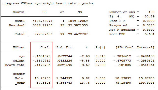
Unstandardized coefficients indicate how much the dependent variable varies with an independent variable, when all other independent variables are held constant. Consider the effect of age in this example. The unstandardized coefficient, B₁, for age is equal to -0.165 (see the first row of the Coef. column). This means that for each 1 year increase in age, there is a decrease in VO₂max of 0.165 ml/min/kg.

Statistical significance of the independent variables

You can test for the statistical significance of each of the independent variables. This tests whether the unstandardized (or standardized) coefficients are equal to 0 (zero) in the population. If p < .05, you can conclude that the coefficients are statistically significantly different to 0 (zero). The t-value and corresponding p-value are located in the "t" and "P>|t|" columns, respectively, as highlighted below:

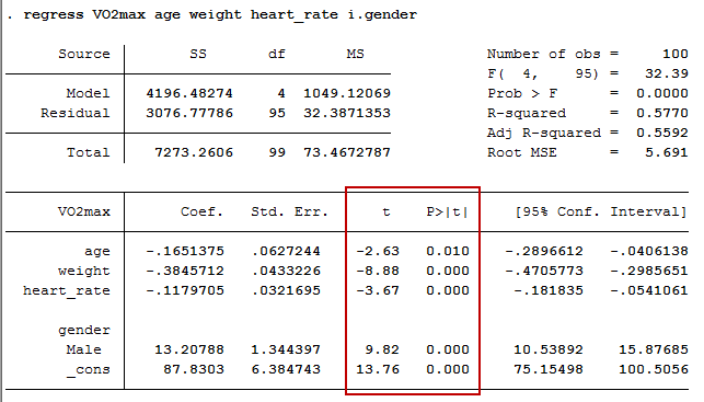
You can see from the "P>|t|" column that all independent variable coefficients are statistically significantly different from 0 (zero). Although the intercept, B₀, is tested for statistical significance, this is rarely an important or interesting finding.

Stata

Reporting the output of multiple regression analysis

You could write up the results as follows: