Binomial Logistic Regression Analysis using Stata

Introduction

A binomial logistic regression is used to predict a dichotomous dependent variable based on one or more continuous or nominal independent variables. It is the most common type of logistic regression and is often simply referred to as logistic regression. In Stata they refer to binary outcomes when considering the binomial logistic regression. It many ways a binomial logistic regression can be considered as a multiple linear regression, but for a dichotomous rather than a continuous dependent variable.

For example, you could use a binomial logistic regression to understand whether dropout of first-time marathon runners (i.e., failure to finish the race) can be predicted from the duration of training performed, age, and whether participants ran for a charity. Dropout is the dichotomous dependent variable (i.e., "completed" or "dropped out"). Duration of training (in months), age (in years) and charity ("yes" or "no") are the independent variables. Another example where you could use a binomial logistic regression is to understand whether the premature failure of a new type of light bulb (i.e., before its one year warranty) can be predicted from the total duration the light is on for, the number of times the light is switched on and off, and the temperature of the ambient air. In this case, premature failure is the dichotomous dependent variable (i.e., the light bulb fails within its one year warranty: "yes" or "no"). The other three variables used to predict the light bulb failure are all continuous independent variables: the total duration the light is on for (in minutes), the number of times the light is switched on and off and the ambient air temperature (in °C).

This "quick start" guide shows you how to carry out a binomial logistic regression using Stata, as well as how to interpret and report the results from this test. However, before we introduce you to this procedure, you need to understand the different assumptions that your data must meet in order for binomial logistic regression to give you a valid result. We discuss these assumptions next.

Note: We do not currently have a premium version of this guide in the subscription part of our website. If you would like us to add a premium version of this guide, please contact us.

Stata

Assumptions

There are six assumptions that underpin binomial logistic regression. If any of these six assumptions are not met, you might not be able to analyse your data using a binomial logistic regression because you might not get a valid result. Since assumptions #1 and #2 relate to your choice of variables, they cannot be tested for using Stata. However, you should decide whether your study meets these assumptions before moving on.

• Assumption #1: Your dependent variable should consist of two categorical, independent (unrelated) groups (i.e., a dichotomous variable). Examples of dichotomous variables include gender (2 groups: male or female), treatment type (2 groups: medication or no medication), educational level (2 groups: undergraduate or postgraduate), religious (2 groups: yes or no), and so forth. If you are unsure whether your dependent variable is dichotomous, see our Types of Variable guide. The two categories of the dependent variable need to be mutually exclusive and exhaustive.
• Assumption #2: You have two or more independent variables, which should be measured at the continuous or nominal level. Examples of continuous variables include height (measured in feet and inches), temperature (measured in °C), salary (measured in US dollars), revision time (measured in hours), intelligence (measured using IQ score), reaction time (measured in milliseconds), test performance (measured from 0 to 100), sales (measured in number of transactions per month), and so forth. Examples of nominal variables include gender (e.g., 2 groups: male and female), ethnicity (e.g., 3 groups: Caucasian, African American and Hispanic), profession (e.g., 5 groups: surgeon, doctor, nurse, dentist, therapist), and so forth.

  Note: Ordinal independent variables can be used, but they must be treated as either continuous or nominal variables. However, you can treat some ordinal variables as continuous and some as nominal; they do not all have to be treated the same. Examples of ordinal variables include Likert items (e.g., a 7-point scale from "strongly agree" through to "strongly disagree"), amongst other ways of ranking categories (e.g., a 3-point scale explaining how much a customer liked a product, ranging from "Not very much", to "It is OK", to "Yes, a lot").

Fortunately, you can check assumptions #3, #4, #5 and #6 using Stata. Do not be surprised if your data fails one or more of these assumptions since this is fairly typical when working with real-world data rather than textbook examples, which often only show you how to carry out a binomial logistic regression when everything goes well. However, don’t worry because even when your data fails certain assumptions, there is often a solution to overcome this (e.g., transforming your data or using another statistical test instead). Just remember that if you do not check that you data meets these assumptions or you test for them incorrectly, the results you get when running a binomial logistic regression might not be valid.

• Assumption #3: You should have independence of observations, which means that there is no relationship between the observations. If you do not have independence of observations, you most likely have repeated measures, and you will need another type of statistical test.
• Assumption #4: Your data must not show multicollinearity, which occurs when you have two or more independent variables that are highly correlated with each other.
• Assumption #5: There needs to be a linear relationship between any continuous independent variables and the logit transformation of the dependent variable.
• Assumption #6: There should be no significant outliers, high leverage points or highly influential points, which represent observations in your data set that are in some way unusual. These can have a very negative effect on the binomial logistic regression equation that is used to predict the value of the dependent variable based on the independent variables. You can check for outliers, leverage points and influential points using Stata.

In practice, checking for assumptions #3, #4, #5 and #6 will probably take up most of your time when carrying out a binomial logistic regression. However, it is not a difficult task, and Stata provides all the tools you need to do this.

In the section, Test Procedure in Stata, we illustrate the Stata procedure required to perform a binomial logistic regression assuming that no assumptions have been violated. First, we set out the example we use to explain the binomial logistic regression procedure in Stata.

Stata

Example

A teacher wanted to understand whether the number of hours students' spent revising predicted success in their final year exams. They also questioned whether gender would influence exam success (although they didn't expect that it would). Therefore, the teacher recruited 189 students who were about to undertake their final year exams. The teacher had the students estimate the numbers of hours they spent revising and record their gender. He then gained their final year exam marks to discover whether they passed or failed the exam. In order to understand whether the number of hours of study had an effect on passing the exam, the teacher ran a binomial logistic regression. Therefore, in this example, the dichotomous dependent variable is pass, which has two categories: "passed" and "failed". The number of hours of study was a continuous independent variable, hours (in hours), and the gender of a participant was a dichotomous independent variable, gender, with two categories: "Male" and "Female".

Note: The example and data used for this guide are fictitious. We have just created them for the purposes of this guide.

Stata

Setup in Stata

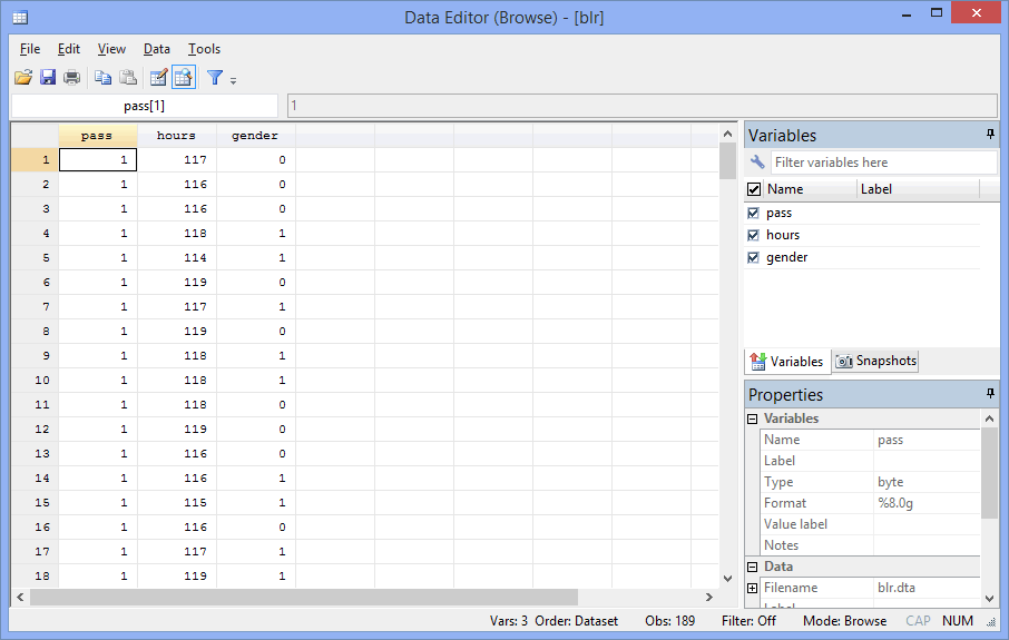
In Stata, we created three variables: (1) pass, which is coded "1" for those who passed the exam and "0" for those who did not pass the exam (i.e., the dependent variable); (2) hours, which is the number of hours studied; and (3) gender, which is the participant's gender (i.e., the last two are the independent variables).

After creating these three variables, we entered the scores for each into the three columns of the Data Editor (Edit) spreadsheet, as shown below:

Published with written permission from StataCorp LP.

Stata

Test Procedure in Stata

In this section, we show you how to analyze your data using a binomial logistic regression in Stata when the six assumptions in the previous section, Assumptions, have not been violated. You can carry out binomial logistic regression using code or Stata's graphical user interface (GUI). After you have carried out your analysis, we show you how to interpret your results. First, choose whether you want to use code or Stata's graphical user interface (GUI).

Code

The code to carry out a binomial logistic regression on your data takes the form:

logistic DependentVariable IndependentVariable#1 IndependentVariable#2 IndependentVariable#3 IndependentVariable#4

This code is entered into the box below:

Using our example where the dependent variable is pass and the two independent variables are hours and gender, the required code would be:

logistic pass hours i.gender

Note: You'll see from the code above that continuous independent variables are simply entered "as is", whilst categorical independent variables have the prefix "i" (e.g., hours for hours, since this is a continuous independent variable, but i.gender for gender, since this is a categorical independent variable).

Therefore, enter the code, logistic pass hours i.gender, and press the "Return/Enter" key on your keyboard.

You can see the Stata output that will be produced here.

Graphical User Interface (GUI)

The six steps required to carry out binomial logistic regression in Stata are shown below:

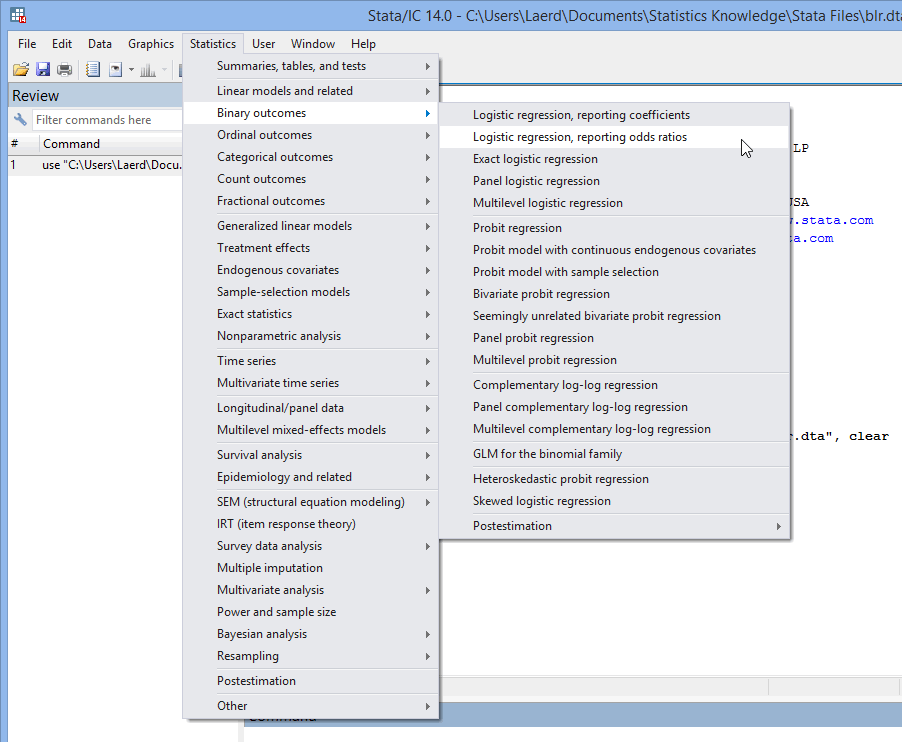
1. Click Statistics > Binary outcomes > Logistic regression, reporting odds ratios on the main menu, as shown below:
   

   Published with written permission from StataCorp LP.

   
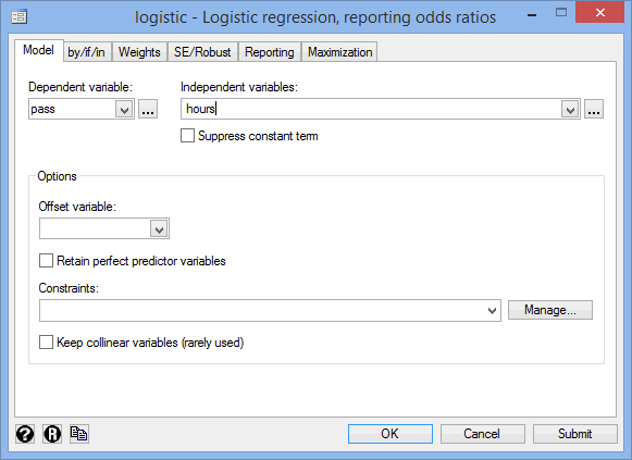
   You will be presented with the logistic - Logistic regression, reporting odds ratios dialogue box, as shown below:
   
   

   Published with written permission from StataCorp LP.

2. Select the dependent variable, pass, from the Dependent variable: drop-down box, and select the continuous independent variable, hours, from the Independent variables: drop-down box, using the relevant buttons. You will be presented with the dialogue box below:
   

   Published with written permission from StataCorp LP.

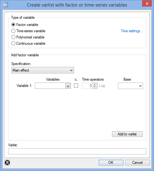
3. Click on the button. You will be presented with the Create varlist with factor or time-series variables dialogue box, as shown below:
   

   Published with written permission from StataCorp LP.

4. Leave Factor variable selected in the –Type of variable– area. Next, in the –Add factor variable– area, leave selected in the Specification: drop-down box. Now, select gender in the Variables drop-down box using the button. Finally, click on the button. You will be presented with the following dialogue box where the categorical independent variable, i.gender, has been entered into the Varlist: box:
   

   Published with written permission from StataCorp LP.

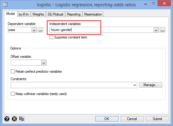
5. Click on the button. You will be returned to the logistic - Logistic regression, reporting odds ratios dialogue box, but with the categorical independent variable, i.gender, now also entered into the Independent variables: box, as shown below:
   

   Published with written permission from StataCorp LP.

6. Click on the button. This will generate the output.

Stata

Output of the binomial logistic regression in Stata

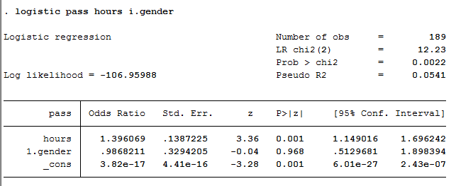
The output below is only a fraction of the options that you have in Stata to analyse your data, assuming that your data passed all the assumptions (e.g., there were no significant influential points), which we explained earlier in the Assumptions section. However, the following output will present the results needed to ascertain whether the independent variables statistically significantly predict the passing of a final year exam. The results are presented under the "Logistic Regression" header, as shown below:

Published with written permission from StataCorp LP.

You can determine whether gender and hours spent revising statistically significantly predicted passing a final year exam by consulting the "P>|z|" column for the "1.gender" and "hours" rows, respectively. The "P>|z|" column contains the p-value for each coefficient and the constant (both expressed as odds ratios). You can see that hours spent revising was statistically significant (i.e., p = .001), but gender was not statistically significant (i.e., p = .968).

Stata

Reporting the output of a binomial logistic regression

When you report the output of your binomial logistic regression, it is good practice to include:

• A. An introduction to the analysis you carried out (e.g., state that you ran a binomial logistic regression).
• B. Information about your sample, including any missing values (e.g., sample size).
• C. An examination of all the assumptions of the binomial logistic regression, including any remedies that were taken for violations of any of these assumptions.
• D. The use of measures, such as the Hosmer-Lemeshow test, to assess how well the model fits the data.
• E. The regression coefficients and/or odds ratios for your binomial logistic regression model, including which are statistically significant, and 95% confidence intervals.

You could write up the results as follows: