Unadjusted versus adjusted means
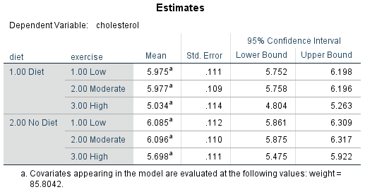
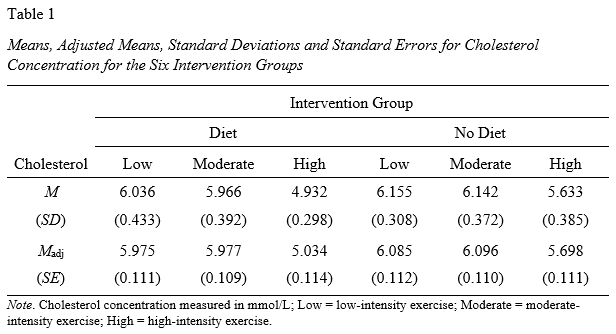
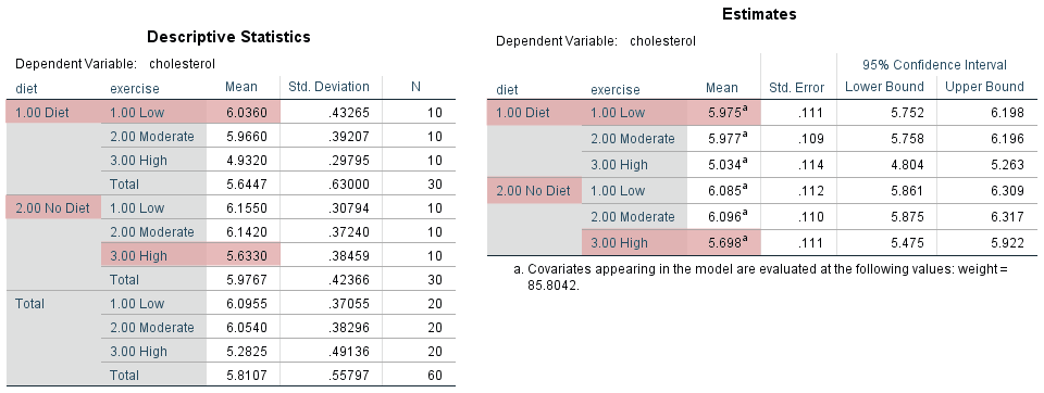
In a two-way ANCOVA analysis, the covariate is included to provide a better assessment of the differences between the groups of the two independent variables in terms of the dependent variable. This is highlighted when comparing the values of the unadjusted means and adjusted means from the Descriptive Statistics and Estimates tables respectively. Therefore, in the diagram below, we have presented the Descriptive Statistics and Estimates tables side-by-side:

For example, start by looking at the first cell of our design in the Descriptive Statistics and Estimates tables above, which reflects participants who dieted and underwent the low-intensity exercise programme (i.e., the row highlighted as "1.00 Diet" and "1.00 Low"). In the Descriptive Statistics table on the left, the unadjusted mean cholesterol concentration for this group was 6.0360 mmol/L, whereas when adjusted for the continuous covariate, weight, the adjusted mean cholesterol concentration was 5.975 mmol/L (i.e., in the Estimates table). In other words, the cholesterol concentration for this group was .061 mmol/L lower when the initial weight of participants was taken into account. Next, look at the sixth cell of our design, which reflects participants who did not diet and underwent the high-intensity exercise programme (i.e., the row highlighted as "2.00 No Diet" and "3.00 High"). In the Descriptive Statistics table on the left, the unadjusted mean cholesterol concentration for this group was 5.6330 mmol/L, whereas when adjusted for the continuous covariate, weight, the adjusted mean cholesterol concentration was 5.698 mmol/L (i.e., in the Estimates table). In other words, the cholesterol concentration for this group was .065 mmol/L higher when the initial weight of participants was taken into account.
Not only were the unadjusted means and adjusted means different in these two cells of our design, but the impact of the covariate, weight, was also different between these two cells (i.e., taking weight into account led to a lower mean cholesterol concentration for participants who dieted and underwent the low-intensity exercise programme, whereas it led to a higher mean cholesterol concentration for participants who did not diet and underwent the high-intensity exercise programme). Whether these differences are important will vary from study to study. For example, is a difference in mean cholesterol concentration .065 mmol/L clinically important? Is an increase or decrease in mean cholesterol concentration when the covariate is taken into account clinically (or practically) important? Is the role that weight has played in terms of showing a higher adjusted mean cholesterol concentration in one group (e.g., participants who dieted and underwent the low-intensity exercise programme) compared to another group (e.g., participants who did not diet and underwent the high-intensity exercise programme) interesting or important in some way? These are the types of questions you might want to ask yourself when evaluating the differences in unadjusted means and adjusted means from the Descriptive Statistics and Estimates tables respectively.
Now that you have an overall impression of your data you can interpret the main result from the two-way ANCOVA (i.e., whether you have a statistically significant two-way interaction effect), which is discussed in the next section.
SPSS Statistics
Determining whether a two-way interaction effect exists
The primary goal of running a two-way ANCOVA is to determine whether there is an interaction effect between the two independent variables, diet and exercise, in terms of the dependent variable, cholesterol, after controlling for the covariate, weight (i.e., whether a two-way interaction effect exists). As we stated on the previous page, in this guide we do not distinguish between a focal variable and moderator variable, but instead investigate: (a) the effect of diet on exercise in terms of cholesterol, after controlling for weight; and (b) the effect of exercise on diet in terms of the cholesterol, after controlling for weight. However, if you are unsure in your own example whether to make such a distinction, please see the brief explanatory note below:
Explanation: In this example, if we were primarily interested in the effect of exercise on differences in adjusted mean cholesterol concentration and wanted to know how this effect might be different if a diet was also undertaken, we would consider exercise to be an example of where we consider one of the independent variables (i.e., exercise) to be the focal variable and the other independent variable (i.e., diet) to be the moderator variable. That is, we are primarily interested in how the effect of exercise on adjusted mean cholesterol concentration is moderated by diet. This is purely a theoretical issue because an interaction effect is symmetrical. That is, an interaction allows the effect of independent variable A to be dependent on independent variable B and vice-versa, independent variable B to be dependent on independent variable A. You can investigate either A on B, B on A, or both. The statistical result you get for the interaction effect does not demand that you investigate A on B or B on A; either or both are permissible. However, theoretically, you might consider one of the independent variables as a focal variable and the other independent variable as a moderator variable. In this situation, the effect of the focal variable is your primary concern, but you think that its effect on the dependent variable depends on the value of the moderator variable. Considering your study in this way has implications not only on how you might interpret and report the two-way ANCOVA result, but also how you might go about analysing a statistically significant result with post hoc tests (Jaccard, 1998).
You can gain an initial impression of whether there is an interaction effect between the two independent variables by visually inspecting the profile plots that were created when you ran the two-way ANCOVA procedure on the previous page. However, a formal statistical test is required to test for the presence of an interaction effect (i.e., via statistical significance testing). Therefore, we first show you how to interpret the two-way interaction effect using these profile plots before explaining how to interpret the two-way interaction effect using a formal statistical test.
Interpreting the two-way interaction effect using profile plots
When plotted, there can be a number of ways in which the two independent variables can be related. However, simply put, if the lines are not parallel (i.e., if they have different patterns or they cross or overlap each other) you might have an interaction effect. Alternatively, if the lines are parallel, you would not expect to have an interaction effect.
Important: Despite the usefulness of profile plots in understanding your data, you cannot determine an interaction effect from them because the profile plot is based on the sample data you have collected and you are interested in determining whether there is an interaction effect in the population from which the sample has been drawn (Fox, 2008). That is, any non-parallel lines in the profile plot might be a consequence of sampling error and not reflect non-parallel lines in the population. Therefore, a formal statistical test is required to test for the presence of an interaction effect (i.e., via statistical significance testing). This is why we use words like might when discussing what a profile plot shows (e.g., as stated above, "If the lines are not parallel...you might have an interaction effect"). That said, the profile plots are still very useful in getting an initial impression of your data and are particularly useful when deciding how to follow up a statistically significant two-way interaction (i.e., whether to interpret and report main effects in addition to simple main effects), which we discuss in our more comprehensive 28 page two-way ANCOVA guide (N.B., you can access this more comprehensive guide by subscribing to Laerd Statistics).
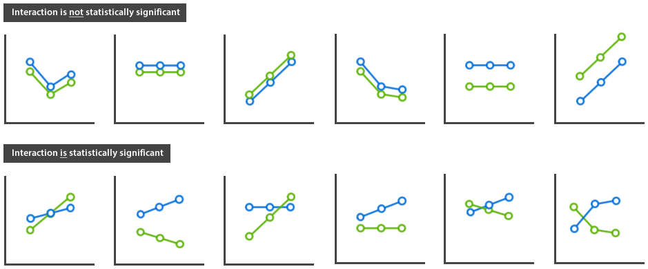
To get an idea of what you are looking for in your profile plot, the diagram below shows you some different possible patterns of the adjusted means and whether they are likely to indicate that a statistically significant two-way interaction effect is present:

Published with written permission from SPSS Statistics, IBM Corporation.
You can see from the diagrams in the top row above that when the lines are parallel, even when there is some distance between them, the two-way interaction effect is not likely to be statistically significant. On the other hand, when the lines take different courses (i.e., are not parallel), whether separated or not, as shown in the diagrams in the bottom row, the two-way interaction effect is likely to be statistically significant. Therefore, look at the two profile plots we generated for our example, as shown below:

Published with written permission from SPSS Statistics, IBM Corporation.
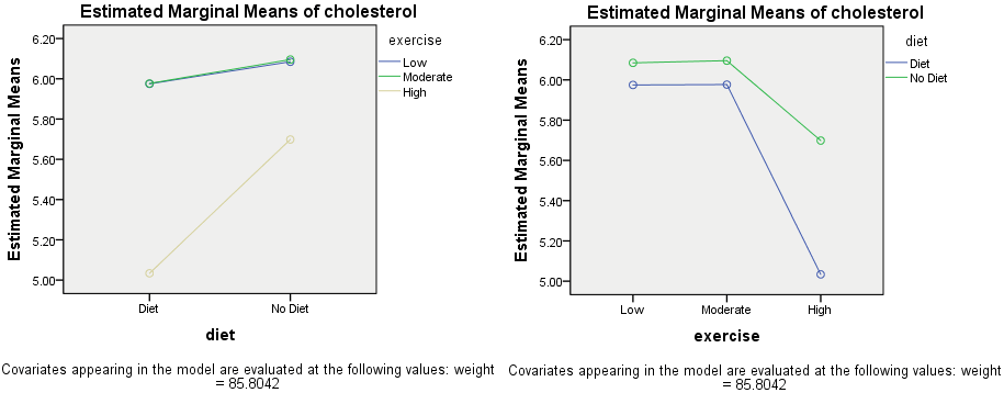
Explanation: There are two profile plots above because when running the main GLM Univariate procedure on the previous page we requested that the two independent variables should be plotted in two ways: (a) diet versus exercise; and (b) exercise versus diet. Therefore, in the profile plot on the left above, diet is shown on the x-axis and exercise is shown by the separate lines. As such, the opposite is plotted in the profile plot on the right above: exercise is shown on the x-axis and diet is shown by the separate lines. Even though the lines in the two profile plots look very different, they are plotting the same data; just in two different ways (i.e., the two independent variables have simply been swapped between the x-axis and the separate lines). We do this because it gives you two opportunities to look at the pattern of the lines in the profile plots; that is, it gives you a better appreciation of the trends in the data, as recommended by Faraway (2015). This makes it easier to decide whether the lines are parallel (i.e., not likely to be statistically significant) or not parallel (i.e., likely to be statistically significant).
Note: If you choose to include the profile plots above in your results section, we would recommend at least correcting the scale of the y-axis. When creating these profile plots, SPSS Statistics does its best to create a suitable scale, but since it does not know what your dependent variable represents it may not use an appropriate scale. In our example, the y-axis ranges between 5.00 mmol/L and 6.20 mmol/L, which is fine. However, the range chosen by SPSS Statistics may not be a suitable range when your data is plotted.
The profile plot on the right is similar in orientation to the example profiles plots illustrated earlier on this page (i.e., on the bottom row). You can see that the two lines are not parallel and do not cross. The same is the case for the profile plot on the left. The three lines do not cross and only two of the three are parallel. Therefore, the two-way interaction effect between diet and exercise might be statistically significant. However, this only tells us half of the story. The pattern of the lines – that is, whether the lines cross or do not cross – tells us about the nature of the interaction; that is, whether the interaction is ordinal or disordinal. When lines do not cross, you have what is called an ordinal interaction. On the other hand, if the lines do cross, you have a disordinal interaction. Since the lines do not cross in our example, this suggests that we have an ordinal interaction.
Whilst it is important to determine whether the two-way interaction effect might be statistically significant and what the nature of this interaction is (i.e., ordinal or disordinal), we also need to understand what the two profile plots show in terms of our example. This interpretation is made easier because we generated two profile plots: (a) one for diet versus exercise; and (b) one for exercise versus diet. Therefore, refer back to the two profile plots we generated for our example below:

Published with written permission from SPSS Statistics, IBM Corporation.
Overall, it would appear that diet has a similar impact on post-intervention cholesterol concentration when undertaken in addition to a low-intensity and moderate-intensity exercise training programme, but has a much larger impact when combined with a high-intensity exercise training programme. This is highlighted by looking at each profile plot in turn: (a) diet versus exercise; and (b) exercise versus diet.
- Diet versus exercise: The profile plot on the left above is useful in clearly distinguishing the lower cholesterol concentrations for participants who were in the high-intensity exercise programme (i.e., the beige line) compared to the low-intensity and moderate-intensity exercise programmes (i.e., the blue and green lines). There is also a clear difference in the slope of the lines when comparing the diet and no diet groups who underwent one of the three exercise intensity programmes. For example, the difference in cholesterol concentrations for participants who were in the low-intensity and moderate-intensity exercise programmes appears relatively small between the diet and no diet groups compared to the difference in cholesterol concentrations for participants in the diet and no diet groups who were in the high-intensity exercise programme (i.e., the blue and green lines of the low- and moderator-intensity exercise programmes are relatively shallow between the diet and no diet programmes compared to the steeper beige line of the high-intensity exercise programme). As such, the profile plot of diet versus exercise on the left above would suggest that the two-way interaction effect exists, or is most strong, for the interaction of diet with the high-intensity exercise training programme.
- Exercise versus diet: When inspecting the profile plot on the right above, this is useful because it clearly shows how cholesterol concentrations were lower for participants in the diet programme (i.e., the blue line) compared to the no diet programme (i.e., the green line) in all three exercise programmes (i.e., in the low-, moderate- and high-intensity exercise programmes that are now shown along the x-axis). Also, whereas the lines are not far from parallel when comparing participants in the diet and no diet groups who also underwent the low-intensity and high-intensity exercise programmes, the lines clearly diverge (i.e., are not parallel) when comparing the diet and no diet groups who underwent the high-intensity exercise programme. As such, the profile plot of exercise versus diet on the right above would suggest that the two-way interaction effect exists, or is most strong, for the interaction of diet with the high-intensity exercise training programme.
Therefore, profile plots can be very useful not only in showing where there might be a two-way interaction effect, but also in describing and highlighting possible patterns in our data. Furthermore, determining whether you have an ordinal interaction or disordinal interaction has important implications on how you follow-up a statistically significant interaction effect (i.e., whether you might report main effects in addition to simple main effects), which is discussed in our more comprehensive two-way ANCOVA guide. However, we must stress that the profile plots reflect our sample data and not the population we have drawn our sample from. Therefore, a formal statistical test is required to test for the presence of a two-way interaction effect (i.e., via statistical significance testing), which is discussed in the next section.
Interpreting the two-way interaction effect using a formal statistical test
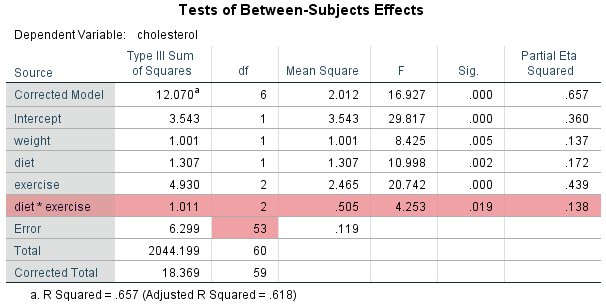
You can determine whether you have a statistically significant two-way interaction effect by interpreting the Tests of Between-Subjects Effects table. The interaction effect is represented as the product of the two independent variables in a two-way ANCOVA (i.e., independent variable A x independent variable B), but with the multiplication sign (i.e., "x") being replaced with an asterisk in SPSS Statistics (i.e., "*"). Therefore, the two-way interaction effect in our example is labelled "diet * exercise". As such, you need to interpret the "diet * exercise" row in the Tests of Between-Subjects Effects table, as highlighted below:

Published with written permission from SPSS Statistics, IBM Corporation.
The "Sig." column presents the significance value (i.e., p-value) of the two-way interaction effect. If p < .05 (i.e., if p is less than .05), you have a statistically significant two-way interaction effect. Alternatively, if p > .05 (i.e., if p is greater than .05), you do not have a statistically significant two-way interaction effect.
You can see from the highlighted row above that the p-value for this interaction effect is .019 (i.e., p = .019). Since .019 is less than .05 (i.e., it satisfies p < .05), this means that there is a statistically significant two-way interaction effect. It indicates that we were correct in thinking that the effect of a diet on cholesterol concentration (after controlling for weight) depends on the exercise programme being undertaken or, equivalently, the effect of an exercise training programme on cholesterol concentration (after controlling for weight) depends on whether the exercise programme is accompanied by a diet.
Note: If you see SPSS Statistics state that the "Sig." value is ".000", this means that p < .0005; it does not mean that the significance level is actually zero. For the APA style, all p-values less than .001 should be written p < .001. When the p-value is greater than .001, it is preferable to state the actual p-value rather than a greater/less than p-value statement (e.g., p = .023 rather than p < .05). This way, you convey more information to the reader about the level of statistical significance of your result.
You could report a statistically significant two-way interaction effect as follows:
There was a statistically significant interaction between diet and exercise on cholesterol concentration, whilst controlling for weight, F(2, 53) = 4.253, p = .019, partial η2 = .138.
There was a statistically significant interaction between diet and exercise on cholesterol concentration, whilst controlling for weight, F(2, 53) = 4.25, p = .019, partial η2 = .138.
In the statement above, the F(2, 53) = 4.253, p = .019, partial η2 = .138 part has the following meaning:
| Column name |
Column meaning |
| F |
Indicates that we are comparing to an F-distribution (F-test). |
| 2 in (2, 53) |
Indicates the degrees of freedom for the interaction term. |
| 53 in (2, 53) |
Indicates the degrees of freedom for the error term. |
| 4.253 (or 4.25 in APA style) |
Indicates the obtained value of the F-statistic (obtained F-value). |
| p = .019 |
Indicates the probability of obtaining the observed F-value given the null hypothesis is true. |
| partial η2 = .138 |
A measure of effect size. |
On the other hand, if p > .05 (i.e., if the p-value is greater than .05), you do not have a statistically significant two-way interaction effect. You could report this result as follows:
There was no statistically significant interaction between diet and exercise on cholesterol concentration, whilst controlling for weight, F(2, 53) = 1.215, p = .432, partial η2 = .020.
There was no statistically significant interaction between diet and exercise on cholesterol concentration, whilst controlling for weight, F(2, 53) = 1.22, p = .432, partial η2 = .02.
Note: The results in the example write-up above have been made up to provide an example of a non-statistically significant result, so you will not find these results in any of the SPSS Statistics output.
Depending on whether you have a statistically significant two-way interaction effect will determine how you should proceed in your analysis (i.e., what follow-up tests you carry out), as discussed in the next section.
SPSS Statistics
Follow-up analysis after determining whether there is a statistically significant two-way interaction effect
As mentioned above, whether you have a statistically significant two-way interaction effect will determine how you follow up your analysis; in other words, what analysis you can carry out next in order to learn more about your data. There are three types of follow-up analysis you can carry out: (a) simple main effects; (b) interaction contrasts; and/or (c) main effects. Whilst there are preferences to which of these three types of result you should interpret depending on whether your two-way interaction term is statistically significant, it is important to take a common sense approach to selecting the most appropriate method.
Generally speaking, if you have a statistically significant interaction effect, you can consider following up your analysis using simple main effects (Jaccard, 1998; Keppel & Wickens, 2004; Kinnear & Gray, 2010; Maxwell & Delaney, 2004) or interaction contrasts. Alternatively, if you do not have a statistically significant interaction effect, you can consider following up your analysis using main effects (e.g., Howell, 2010). Unfortunately, the choice between simple main effects and main effects is not so simple in practice. There are occasions when you may want to report simple main effects when the two-way interaction effect is not statistically significant (Faraway, 2015; Fox, 2008; Searle, 2006). There are also occasions when you may want to report main effects in addition to simple main effects when the two-way interaction effect is statistically significant, but you need to be careful because this can be misleading (Shadish et al., 2002). Due to these challenges in knowing when to carry out and report simple main effects and main effects, we dedicate a section of our more comprehensive 28 page two-way ANCOVA guide to help you understand these options (N.B., you can access this two-way ANCOVA guide by subscribing to Laerd Statistics). Nonetheless, in this introductory guide, we briefly explain what these two types of follow-up analysis – simple main effects and main effects – will help you to learn about your two-way ANCOVA results. Finally, we briefly introduce the IBM SPSS Statistics Syntax Editor that you will need to use to carry out simple main effects using SPSS Statistics.
Simple main effects
In our example, there are five simple main effects. The three simple main effects of diet are:
- Low-intensity exercise group: The effect that dieting versus not dieting has on cholesterol concentration (after controlling for weight) in the low-intensity exercise group.
- Moderate-intensity exercise group: The effect that dieting versus not dieting has on cholesterol concentration (after controlling for weight) in the moderate-intensity exercise group.
- High-intensity exercise group: The effect that dieting versus not dieting has on cholesterol concentration (after controlling for weight) in the high-intensity exercise group.
In terms of exercise, the two simple main effects are:
- Diet group: The effect that undertaking low- versus moderate- versus high-intensity exercise has on cholesterol concentration (after controlling for weight) in the diet group.
- No diet group: The effect that undertaking low- versus moderate- versus high-intensity exercise has on cholesterol concentration (after controlling for weight) in the no diet group.
Therefore, when the two-way interaction effect is statistically significant in a two-way ANCOVA, we investigate whether the differences in adjusted means in each of these five simple main effects is statistically significant. For example, if we take the first simple main effect for diet (i.e., in the first of the five bullets above), we would investigate whether there was a statistically significant difference in the adjusted mean cholesterol concentration between participants who dieted and did not diet who were also in the low-intensity exercise group. This may indicate that, for example, there was relatively little difference in adjusted mean cholesterol concentration between participants who underwent a diet compared to those who did not diet in the low-intensity exercise group. It may also show that this simple main effect was not statistically significant (i.e., there was no difference in adjusted mean cholesterol concentration in the population from which our sample was drawn). However, we must stress that you may also want to interpret main effects in addition to simple main effects.
Main effects
In our example we have two main effects:
- A main effect of diet: A statistically significant main effect of diet indicates that there is a difference in the effect of diet on cholesterol (after controlling for weight) when ignoring (averaging over) the levels of exercise (i.e., taking exercise into account as a whole, but ignoring whether a participant was in the "low-", "moderate-" or "high-intensity" exercise group). In other words, there is a difference in cholesterol concentration (after adjusting for weight) between participants who underwent the diet and no diet programmes when ignoring which exercise programme participants also underwent. Whilst a statistically significant main effect will not tell us where these differences are (e.g., whether cholesterol concentration was higher in the group who dieted compared to the group who did not diet, or vice versa), if the main effect of diet is statistically significant, we can use pairwise comparisons to understand where these specific differences between the groups are.
- A main effect of exercise: A statistically significant main effect of exercise indicates that there is a difference in the effect of exercise on cholesterol (after controlling for weight) when ignoring (averaging over) the levels of diet (i.e., taking diet into account as a whole, but ignoring whether a participant was in the "diet" or "no diet" programme). In other words, there is a difference in cholesterol concentration (after adjusting for weight) between participants who underwent the low-, moderate- or high-intensity exercise programmes when ignoring whether participant also dieted or did not diet. Whilst a statistically significant main effect will not tell us where these differences are (e.g., whether cholesterol concentration was higher in the low-intensity exercise groups compared to the high-intensity exercise group, or vice versa), if the main effect of exercise is statistically significant, we can use pairwise comparisons to understand where these specific differences between the groups are.
Therefore, when the two-way interaction effect is not statistically significant in a two-way ANCOVA, we investigate whether the differences in adjusted marginal means in these two main effects are statistically significant. For example, if we take the main effect for diet (i.e., in the first of the two bullets above), we would investigate whether there was a statistically significant difference in the adjusted marginal mean cholesterol concentration between participants who dieted and those who did not diet. This may indicate that, for example, there was a difference of .298 mmol/L in adjusted marginal mean cholesterol concentration between participants who underwent a diet compared to those who did not diet. It may also show that this main effect was statistically significant (i.e., a difference in adjusted marginal mean cholesterol concentration exists in the population from which our sample was drawn). Again, we must stress in some cases you would still report simple main effects rather than main effects when the two-way interaction effect is not statistically significant.
Carrying out simple main effects using SPSS Statistics
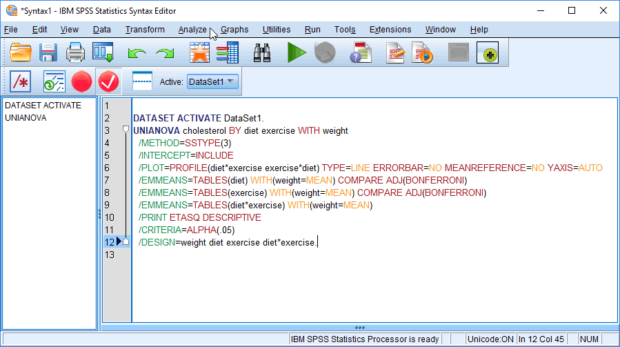
Whilst you can determine whether there was a statistically significant two-way interaction effect, as well as carrying out main effects using the point-and-click system on the previous page, carrying out simple main effects using SPSS Statistics requires syntax (i.e., computer code). This syntax/computer code is entered into the IBM SPSS Statistics Syntax Editor window. For example, the code that was generated for the two-way ANCOVA analysis run on the previous page is highlighted in the IBM SPSS Statistics Syntax Editor window below:

Published with written permission from SPSS Statistics, IBM Corporation.
In order to carry out simple main effects, you need to add to the syntax/computer code above, as well as make a number of changes so that SPSS Statistics understands what simple main effects analysis you want to carry out and how to make an adjustment for multiple comparisons (i.e., the fact that you are running multiple simple main effects on the same data set). If you are not familiar with writing syntax/computer code in SPSS Statistics, we explain how to do this to carry out simple main effects analysis in our more comprehensive two-way ANCOVA guide. We also dedicate a number of pages to help you understand how to interpret the results from your simple main effects, as well as your main effects. You can access this 28 page two-way ANCOVA guide by subscribing to Laerd Statistics (please note that membership includes access to all of our guides).
SPSS Statistics
References
Faraway, J. J. (2015). Linear models with R (2nd ed.). Boca Raton, FL: CRC Press.
Fox, J. (2008). Applied regression analysis and generalized linear models (2nd ed.). Thousand Oaks, CA: Sage Publications.
Huitema, B. E. (2011). The analysis of covariance and alternatives. Hoboken, NJ: Wiley.
Jaccard, J. (1998). Interaction effects in factorial analysis of variance. Thousand Oaks, CA: Sage Publications.
Keppel, G., & Wickens, T. D. (2004). Design and analysis: A researcher's handbook (4th ed.). Upper Saddle River, NJ: Prentice Hall.
Kinnear, P. R., & Gray, C. D. (2010). PASW 17 statistics made simple. New York, NY: Psychology Press.
Maxwell, S. E., & Delaney, H. D. (2004). Designing experiments and analyzing data: A model comparison perspective (2nd ed.). New York, NY: Psychology Press.
Searle, S. R. (2006). Linear models for unbalanced data. Hoboken, NJ: John Wiley & Sons.

