Two-way ANCOVA in SPSS Statistics (page 2)

On the previous page you learnt about the type of research where a two-way ANCOVA can be used and the critical assumptions of the two-way ANCOVA that your study design, variables and data must meet in order for the two-way ANCOVA to be the correct statistical test for your analysis. On this page, we set out the example we use to illustrate the two-way ANCOVA using SPSS Statistics, before showing how to set up your data in the Variable View and Data View of SPSS Statistics. We then demonstrate the SPSS Statistics procedure to carry out a two-way ANCOVA based on whether you have SPSS Statistics version 25, 26 or 27 (or the subscription version of SPSS Statistics) or version 24 or an earlier version of SPSS Statistics, since the procedure is slightly different based on the version of SPSS Statistics you have. Therefore, start by reading the example we use throughout this introductory guide in the next section.

SPSS Statistics

Example used in this introductory two-way ANCOVA guide

If a person is overweight and does not exercise, two important steps that they can take to improve their heart health are to diet (i.e., lose weight) and/or start exercising. A researcher would like to understand how well a diet and exercise programme can improve cholesterol concentration, which is a marker of health. At the same time, the researcher would like to control for a person's weight. Therefore, in this example the dependent variable is cholesterol, the two independent variables are diet and exercise, and the covariate (also known as a control variable) is weight.

The researcher recruited 60 participants to the study. There were three different exercise interventions – a low-intensity, moderate-intensity and high-intensity exercise programme – and there were two dietary interventions: diet and no diet. These two interventions were combined so that participants could be in one of six intervention groups, which are known as the six cells of this study design, as shown below:

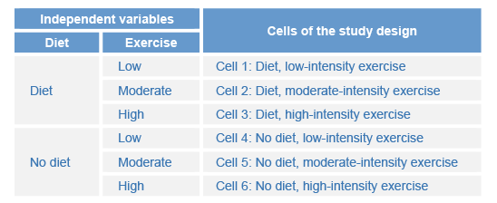
By considering the six groups as two independent variables, diet and exercise, a two-way interaction effect can be established, which allows the researcher to know: (a) whether the effect of diet depends on exercise intensity; and (b) whether the effect of exercise depends on whether a diet is also undertaken.

Participants were randomly assigned to each group so that there were 10 participants in each of the six groups (i.e., 6 x 10 = 60 participants). At the beginning of the interventions the researcher measured participants' weight, weight, which was considered the continuous covariate. After the interventions, cholesterol concentration, cholesterol, was taken as the outcome measure of the study (i.e., the dependent variable).

In order to discover whether the effect of exercise on cholesterol concentration was different if combined with a dietary intervention or no dietary intervention, a two-way ANCOVA was run to primarily assess the statistically significance of the two-way interaction effect. In variable terms, the researcher wanted to know if there was an two-way interaction effect between diet and exercise in terms of cholesterol, whilst controlling for weight.

In this example we do not distinguish between a focal variable and moderator variable, but instead investigate: (a) the effect of diet on exercise in terms of cholesterol, whilst controlling for weight; and (b) the effect of exercise on diet in terms of cholesterol, whilst controlling for weight. However, if you are unsure in your own example whether to make such a distinction, please see the brief explanatory note below.

Explanation: In this example, if we were primarily interested in the effect of exercise on differences in cholesterol concentration and wanted to know how this effect might be different if a diet was also undertaken, we would consider exercise to be an example of where we consider one of the independent variables (i.e., exercise) to be the focal variable and the other independent variable (i.e., diet) to be the moderator variable. That is, we are primarily interested in how the effect of exercise on cholesterol concentration is moderated by diet. This is purely a theoretical issue because an interaction effect is symmetrical. That is, an interaction allows the effect of independent variable A to be dependent on independent variable B and vice-versa, independent variable B to be dependent on independent variable A. You can investigate either A on B, B on A, or both. The statistical result you get for the interaction effect does not demand that you investigate A on B or B on A; either or both are permissible. However, theoretically, you might consider one of the independent variables as a focal variable and the other independent variable as a moderator variable. In this situation, the effect of the focal variable is your primary concern, but you think that its effect on the dependent variable depends on the value of the moderator variable. Considering your study in this way has implications not only on how you might interpret and report the two-way ANCOVA result, but also how you might go about analysing a statistically significant result with post hoc tests (Jaccard, 1998).

SPSS Statistics

Data setup in SPSS Statistics for the two-way ANCOVA

For a two-way ANCOVA with one continuous covariate, you will have four variables. In this example, these are:

(1) The dependent variable, cholesterol, which is cholesterol concentration post-intervention (i.e., cholesterol concentration at the end of the experiment).

(2) The independent variable, diet, which has two groups: "Diet" and "No diet".

(3) The independent variable, exercise, which has three levels: the "Low", "Moderate" and "High" intensity exercise programmes.

(4) The covariate, weight, which is the weight of participants pre-intervention (i.e., participants' weight at the start of/just before the experiment.

Note: The independent variable, exercise, is an ordinal variable, so it is set up as an ordinal variable in SPSS Statistics, but the two-way ANCOVA does not take into account the ordered nature of an ordinal variable.

To set up these four variables, SPSS Statistics has a Variable View where you define the types of variables you are analysing and a Data View where you enter your data for these variables. First, we show you how to setup your two independent variables and then your dependent variable and covariate in the Variable View window of SPSS Statistics. Finally, we show you how to enter your data into the Data View window.

The Variable View in SPSS Statistics

At the end of the setup process, your Variable View window will look like the one below, which illustrates the setup for the dependent variable, the two independent variables and covariate:

Published with written permission from SPSS Statistics, IBM Corporation.

In the Variable View window above, you will have entered four variables: one on each row. For our example, we have put the dependent variable, cholesterol, on row , the two independent variables, diet and exercise on rows and , and the covariate, weight, on row .

Note: The order that you enter your variables into the Variable View is irrelevant. It will simply determine the order of the columns in the Data View, as explained later.

First, look at the nominal and ordinal independent variables, diet and exercise, on rows and respectively, as shown below:

Published with written permission from SPSS Statistics, IBM Corporation.

The name of your independent variables should be entered in the cells under the column (e.g., "diet" in row to represent our nominal independent variable, diet, and "exercise" in row to represent our ordinal independent variable, exercise). There are certain "illegal" characters that cannot be entered into the cell. Therefore, if you get an error message, you can learn what these illegal characters are in our general data setup guide, which you can access by subscribing to Laerd Statistics.

Note: For your own clarity, you can also provide a label for your variables in the column. For example, the label we entered for "diet" was "Diet intervention (two groups)", whilst the label we entered for "exercise" was "Exercise intervention (three levels)".

The cell under the column should contain the information about the groups/levels of your independent variables (e.g., "Diet" and "No diet" for diet and "Low", "Moderate" and "High" for exercise). To enter this information, click into the cell under the column for one of your independent variables. The button will appear in the cell. Click on this button and the Value Labels dialogue box will appear. You now need to give each group/level of your independent variable a "value", which you enter into the Value: box (e.g., "1"), as well as a "label", which you enter into the Label: box (e.g., "Diet"). By clicking the button the coding will appear in the main box (e.g., "1.00 = "Diet" for diet). The setup for both of our independent variables is shown below:

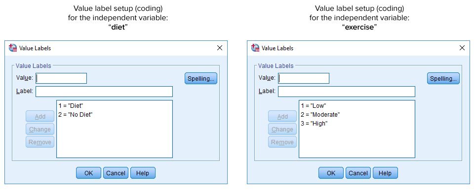
Note: You will typically enter an integer (e.g., "1") into the Value: box to represent the group/level of your independent variable and not a decimal (e.g., "1.00"). However, SPSS Statistics adds 2 decimal places by default when you click on the button (e.g., 1.00 = "Diet"), as shown in the Value Labels box above. Therefore, do not think that you have done anything wrong. We have simply changed the number of decimal places from "2" to "0" in the column above.

The cell under the column should show if you have a nominal independent variable (e.g., diet) and if you have an ordinal independent variable (e.g., exercise). However, just to reiterate, the two-way ANCOVA does not take into account the ordered nature of an ordinal variable. Finally, the cell under the column should show .

Note: We suggest changing the cell under the column from to , but you do not have to make this change. We suggest that you do because there are certain analyses in SPSS Statistics where the setting results in your variables being automatically transferred into certain fields in the dialogue boxes you may use to carry out your analysis. Since you may not want to transfer these variable, we suggest changing the setting to so that this does not happen automatically.

Next, look at the continuous dependent variable, cholesterol, and continuous covariate, weight, on rows and respectively, as shown below:

Published with written permission from SPSS Statistics, IBM Corporation.

The name of your dependent variable and covariate should be entered in the cell under the column (e.g., "cholesterol" and "weight" in our example). The cell under the column should show , indicating that you have a continuous dependent variable and a continuous covariate, whilst the cell under the column should show .

You have now successfully entered all the information that SPSS Statistics needs to know about your dependent variable, two independent variables and covariate into the Variable View window. In the next section, we show you how to enter your data into the Data View window.

The Data View in SPSS Statistics

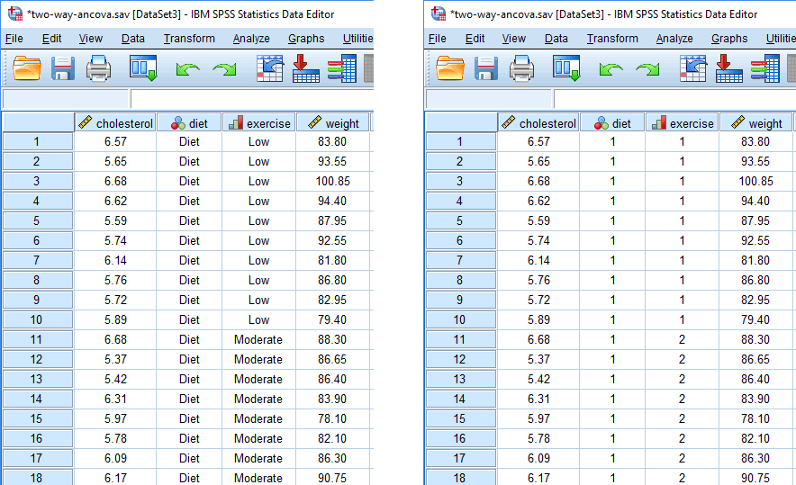
Based on the file setup for the dependent variable, two independent variables and covariate in the Variable View above, the Data View window should look as follows:

Published with written permission from SPSS Statistics, IBM Corporation.

Note: In the Data View above on the left, the responses for the two independent variables are shown in text (e.g., "Diet" under the column and "Low" under the column along row ). In the Data View above on the right, the same responses for the two independent variables are shown using their underlying coding (i.e., "1" for "Diet" and "1" for "Low" along row ). This reflects the coding in the Value Labels dialogue box above: "1" = "Diet" for the nominal independent variable, diet, and "1" = "Low" for the ordinal independent variable, exercise. You can toggle between these two views of your data by clicking the "Value Labels" () icon on the main toolbar.

Your four variables will be displayed in the columns based on the order you entered them into the Variable View window. In our example, we first entered the continuous dependent variable, cholesterol, so this appears in the first column, entitled . Therefore, the second and third columns, and reflects our nominal and ordinal independent variables, diet and exercise, respectively, since these were the second and third variables we entered into the Variable View window. Finally, we entered the continuous covariate, weight, so this appears in the fourth and final column, entitled .

Now, you simply have to enter your data into the cells under each column. Remember that "each row" represents "one case" (e.g., a case could be a single participant). Therefore, in row of our example, our first participant had a cholesterol concentration of 6.57 mmol/L, undertook the diet and low-intensity exercise programmes, and had a weight of 83.80 kg.

Since these cells will initially be empty, you need to click into the cells to enter your data. You'll notice that when you click into the cells under your two independent variables, SPSS Statistics will give you a drop-down option with the groups/levels of the independent variables already populated. However, for your dependent variable and covariate, you simply need to enter the values.

SPSS Statistics

SPSS Statistics procedure for the two-way ANCOVA

The procedure in SPSS Statistics to carry out a two-way ANCOVA is slightly different depending on the version of SPSS Statistics you have. Therefore, in this section we set out the two-way ANCOVA procedure based on whether you have SPSS Statistics version 25, 26 or 27, or the subscription version of SPSS Statistics, or version 24 or earlier versions of SPSS Statistics. These procedures will help you to determine whether you have a statistically significant two-way interaction effect. Based on your result, you would then follow up this result using simple main effects and/or main effects. Carrying out simple main effects and/or main effects requires additional procedures in SPSS Statistics, which we discuss on the next page. First, you need to decide whether you want to run the two-way ANCOVA using SPSS Statistics version 25, 26 or 27 (or the subscription version of SPSS Statistics) or version 24 or an earlier version of SPSS Statistics. The latest versions of SPSS Statistics are version 27 and the subscription version. If you are unsure which version of SPSS Statistics you are using, see our guide: Identifying your version of SPSS Statistics.

SPSS Statistics versions 25, 26 and 27
(and the subscription version of SPSS Statistics)

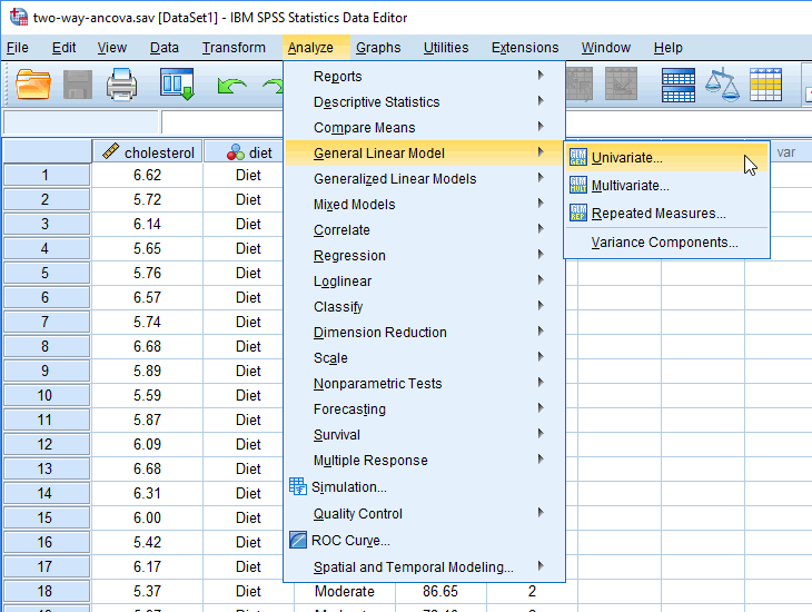
1. Click Analyze > General Linear Model > Univariate... on the main menu, as shown below:

   Note: In version 27 and the subscription version, SPSS Statistics introduced a new look to their interface called "SPSS Light", replacing the previous look for versions 26 and earlier versions, which was called "SPSS Standard". Therefore, if you have SPSS Statistics version 27 or the subscription version of SPSS Statistics, the images that follow will be light grey rather than blue. However, the procedure is identical.

   

   Published with written permission from SPSS Statistics, IBM Corporation.

   
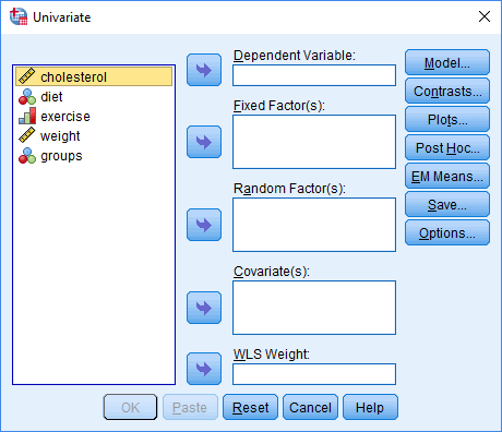
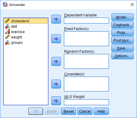
   You will be presented with the Univariate dialogue box, as shown below:
   
   

   Published with written permission from SPSS Statistics, IBM Corporation.

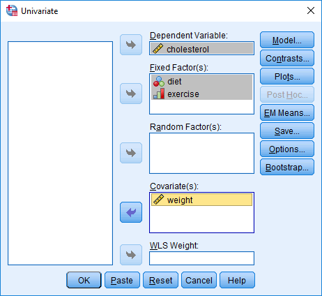
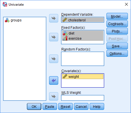
2. Transfer the dependent variable, cholesterol, into the Dependent Variable: box, the two independent variables, diet and exercise, into the Fixed Factor(s): box, and the covariate, weight, into the Covariate(s): box, using the relevant buttons. You will end up with the following screen:
   

   Published with written permission from SPSS Statistics, IBM Corporation.

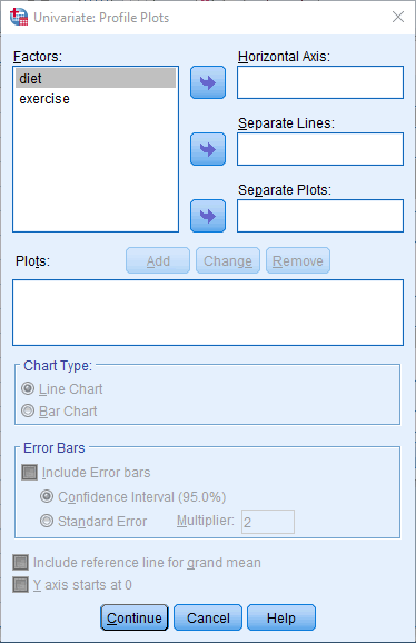
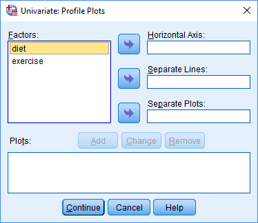
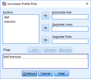
3. Click on the button and you will be presented with the Univariate: Profile Plots dialogue box, as shown below:
   

   Published with written permission from SPSS Statistics, IBM Corporation.

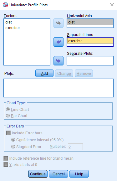
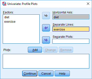
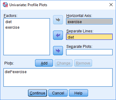
4. Transfer diet from the Factors: box to the Horizontal Axis: box and exercise into the Separate Lines: box, as shown below:
   

   Published with written permission from SPSS Statistics, IBM Corporation.

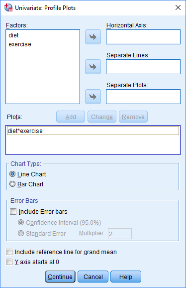
5. Click on the button. This will add this profile plot, which it labels "diet*exercise", into the Plots: box, as shown below:
   

   Published with written permission from SPSS Statistics, IBM Corporation.

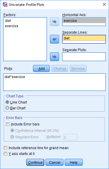
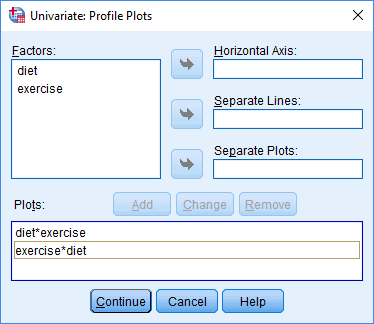
6. Transfer exercise from the Factors: box to the Horizontal Axis: box and diet into the Separate Lines: box, as shown below:
   

   Published with written permission from SPSS Statistics, IBM Corporation.

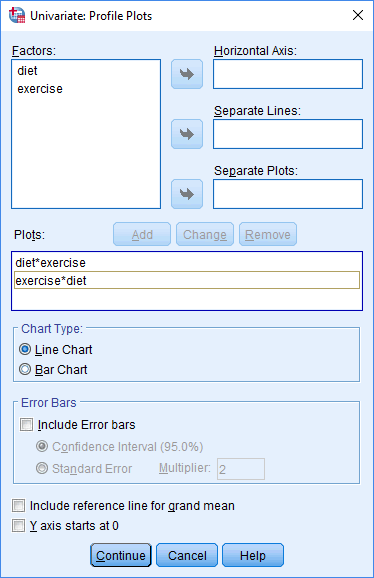
7. Click on the button. This will add this profile plot, which it labels "exercise*diet", into the Plots: box, as shown below:
   

   Published with written permission from SPSS Statistics, IBM Corporation.

8. Click on the button. You will be returned to the Univariate dialogue box.
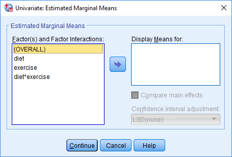
9. Click on the button. You will be presented with the Univariate: Estimated Marginal Means dialogue box, as shown below:
   

   Published with written permission from SPSS Statistics, IBM Corporation.

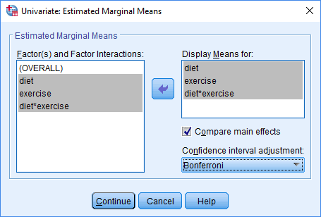
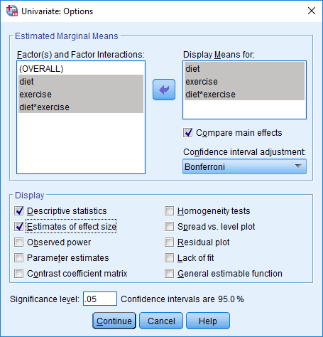
10. Transfer the two independent variables, diet and exercise, as well as the interaction term, diet*exercise, from the Factor(s) and Factor Interactions box into the Display Means for: box using the button. Next, select Compare main effects, which will activate the Confidence interval adjustment: option. From this drop-down menu, select from the options.
    

    Published with written permission from SPSS Statistics, IBM Corporation.

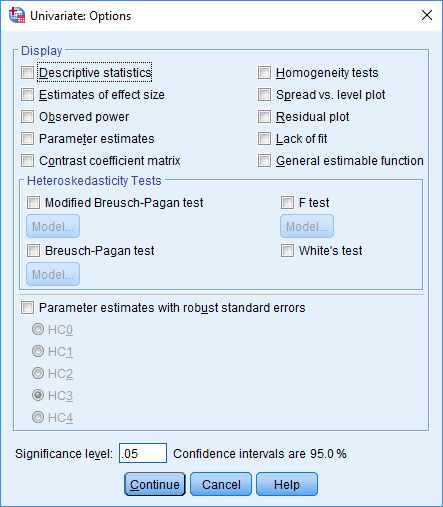
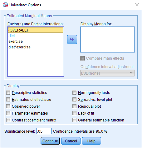
11. Click on the button. You will be presented with the Univariate: Options dialogue box, as shown below:
    

    Published with written permission from SPSS Statistics, IBM Corporation.

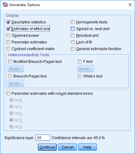
12. Select Descriptive statistics and Estimates of effect size in the –Display– area, as shown below:
    

    Published with written permission from SPSS Statistics, IBM Corporation.

13. Click on the button and you will be returned to the Univariate dialogue box.
14. Click on the button.

How to interpret the SPSS Statistics output when running the two-way ANCOVA procedure is explained on the next page. You can ignore the following section, which shows how to carry out a two-way ANCOVA using SPSS Statistics version 24 and earlier versions of SPSS Statistics.