Repeated Measures ANOVA
Introduction
Repeated measures ANOVA is the equivalent of the one-way ANOVA, but for related, not independent groups, and is the extension of the dependent t-test. A repeated measures ANOVA is also referred to as a within-subjects ANOVA or ANOVA for correlated samples. All these names imply the nature of the repeated measures ANOVA, that of a test to detect any overall differences between related means. There are many complex designs that can make use of repeated measures, but throughout this guide, we will be referring to the most simple case, that of a one-way repeated measures ANOVA. This particular test requires one independent variable and one dependent variable. The dependent variable needs to be continuous (interval or ratio) and the independent variable categorical (either nominal or ordinal).
When to use a Repeated Measures ANOVA
We can analyse data using a repeated measures ANOVA for two types of study design. Studies that investigate either (1) changes in mean scores over three or more time points, or (2) differences in mean scores under three or more different conditions. For example, for (1), you might be investigating the effect of a 6-month exercise training programme on blood pressure and want to measure blood pressure at 3 separate time points (pre-, midway and post-exercise intervention), which would allow you to develop a time-course for any exercise effect. For (2), you might get the same subjects to eat different types of cake (chocolate, caramel and lemon) and rate each one for taste, rather than having different people taste each different cake. The important point with these two study designs is that the same people are being measured more than once on the same dependent variable (i.e., why it is called repeated measures).
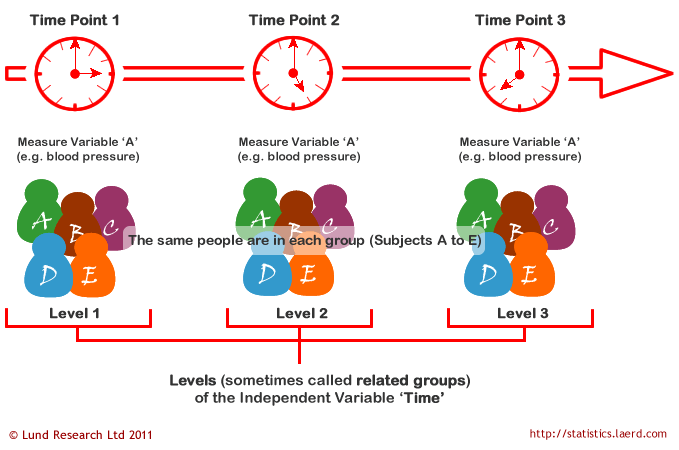
In repeated measures ANOVA, the independent variable has categories called levels or related groups. Where measurements are repeated over time, such as when measuring changes in blood pressure due to an exercise-training programme, the independent variable is time. Each level (or related group) is a specific time point. Hence, for the exercise-training study, there would be three time points and each time-point is a level of the independent variable (a schematic of a time-course repeated measures design is shown below):
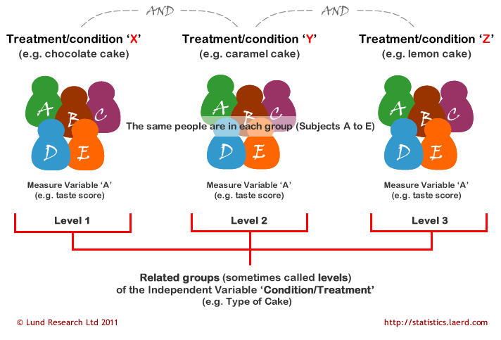
Where measurements are made under different conditions, the conditions are the levels (or related groups) of the independent variable (e.g., type of cake is the independent variable with chocolate, caramel, and lemon cake as the levels of the independent variable). A schematic of a different-conditions repeated measures design is shown below. It should be noted that often the levels of the independent variable are not referred to as conditions, but treatments. Which one you want to use is up to you. There is no right or wrong naming convention. You will also see the independent variable more commonly referred to as the within-subjects factor.
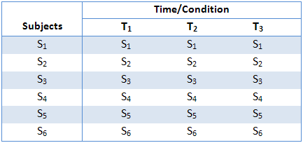
The above two schematics have shown an example of each type of repeated measures ANOVA design, but you will also often see these designs expressed in tabular form, such as shown below:
This particular table describes a study with six subjects (S1 to S6) performing under three conditions or at three time points (T1 to T3). As highlighted earlier, the within-subjects factor could also have been labelled "treatment" instead of "time/condition". They all relate to the same thing: subjects undergoing repeated measurements at either different time points or under different conditions/treatments.
Hypothesis for Repeated Measures ANOVA
The repeated measures ANOVA tests for whether there are any differences between related population means. The null hypothesis (H0) states that the means are equal:
H0: µ1 = µ2 = µ3 = … = µk
where µ = population mean and k = number of related groups. The alternative hypothesis (HA) states that the related population means are not equal (at least one mean is different to another mean):
HA: at least two means are significantly different
For our exercise-training example, the null hypothesis (H0) is that mean blood pressure is the same at all time points (pre-, 3 months, and 6 months). The alternative hypothesis is that mean blood pressure is significantly different at one or more time points. A repeated measures ANOVA will not inform you where the differences between groups lie as it is an omnibus statistical test. The same would be true if you were investigating different conditions or treatments rather than time points, as used in this example. If your repeated measures ANOVA is statistically significant, you can run post hoc tests that can highlight exactly where these differences occur. You can learn how to run appropriate post-hoc tests for a repeated measures ANOVA in SPSS Statistics on page 2 of our guide: One-Way Repeated Measures ANOVA in SPSS Statistics.
Logic of the Repeated Measures ANOVA
The logic behind a repeated measures ANOVA is very similar to that of a between-subjects ANOVA. Recall that a between-subjects ANOVA partitions total variability into between-groups variability (SSb) and within-groups variability (SSw), as shown below:
In this design, within-group variability (SSw) is defined as the error variability (SSerror). Following division by the appropriate degrees of freedom, a mean sum of squares for between-groups (MSb) and within-groups (MSw) is determined and an F-statistic is calculated as the ratio of MSb to MSw (or MSerror), as shown below:
A repeated measures ANOVA calculates an F-statistic in a similar way:
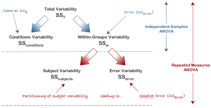
The advantage of a repeated measures ANOVA is that whereas within-group variability (SSw) expresses the error variability (SSerror) in an independent (between-subjects) ANOVA, a repeated measures ANOVA can further partition this error term, reducing its size, as is illustrated below:

This has the effect of increasing the value of the F-statistic due to the reduction of the denominator and leading to an increase in the power of the test to detect significant differences between means (this is discussed in more detail later). Mathematically, and as illustrated above, we partition the variability attributable to the differences between groups (SSconditions) and variability within groups (SSw) exactly as we do in a between-subjects (independent) ANOVA. However, with a repeated measures ANOVA, as we are using the same subjects in each group, we can remove the variability due to the individual differences between subjects, referred to as SSsubjects, from the within-groups variability (SSw). How is this achieved? Quite simply, we treat each subject as a block. That is, each subject becomes a level of a factor called subjects. We then calculate this variability as we do with any between-subjects factor. The ability to subtract SSsubjects will leave us with a smaller SSerror term, as highlighted below:

Now that we have removed the between-subjects variability, our new SSerror only reflects individual variability to each condition. You might recognise this as the interaction effect of subject by conditions; that is, how subjects react to the different conditions. Whether this leads to a more powerful test will depend on whether the reduction in SSerror more than compensates for the reduction in degrees of freedom for the error term (as degrees of freedom go from (n - k) to (n - 1)(k - 1) (remembering that there are more subjects in the independent ANOVA design).
The next page of our guide deals with how to calculate a repeated measures ANOVA.


