ANOVA with Repeated Measures using SPSS Statistics (cont...)
SPSS Statistics version 24
and earlier versions of SPSS Statistics
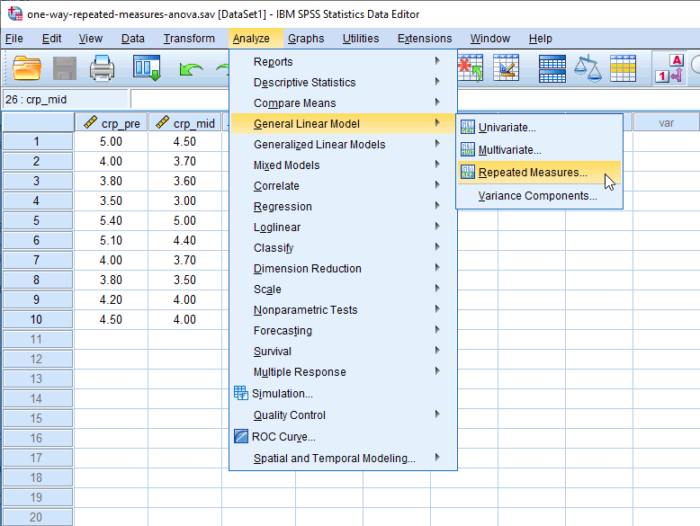
- Click Analyze > General Linear Model > Repeated measures... on the top menu, as shown below:

Published with written permission from SPSS Statistics, IBM Corporation.
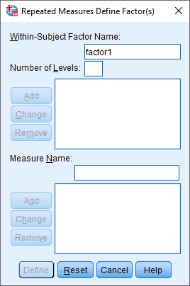
You will be presented with the Repeated Measures Define Factor(s) dialogue box, as shown below:
Published with written permission from SPSS Statistics, IBM Corporation.
Explanation: This dialogue box is where you inform SPSS Statistics that the three variables – crp_pre, crp_mid and crp_post – are three levels of the within-subjects factor, time. Without doing this, SPSS Statistics will think that the three variables are just that, three separate variables.
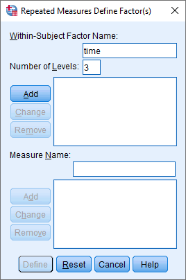
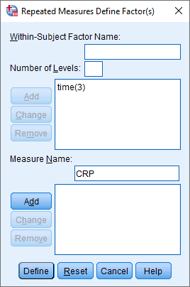
- In the Within-Subject Factor Name: box, replace "factor1" with a more meaningful name for your within-subjects factor. For example, we replaced "factor1" with "time" because this is the name of our within-subjects factor (i.e., time). Next, enter the number of levels of your within-subjects factor into the Number of Levels: box. For example, our within-subjects factor, time, has three levels, representing the three time points when our dependent variable, CRP, was measured (i.e., pre-intervention, crp_pre, mid-intervention, crp_mid, and post-intervention, crp_post). Therefore, we entered "3" into the Number of Levels: box, as shown below:
Published with written permission from SPSS Statistics, IBM Corporation.
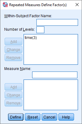
Click on the button and you will be presented with the following screen:
Published with written permission from SPSS Statistics, IBM Corporation.
- In the Measure Name: box, enter a name that reflects the name of your dependent variable. Since our dependent variable is CRP, we entered "CRP", as shown below:
Published with written permission from SPSS Statistics, IBM Corporation.
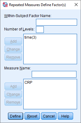
Click on the button and you will get the following screen:
Published with written permission from SPSS Statistics, IBM Corporation.
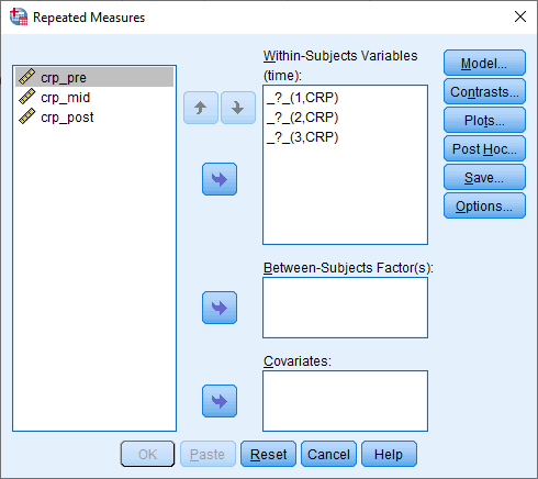
- Click on the button and you will be presented with the Repeated Measures dialogue box, as shown below:
Published with written permission from SPSS Statistics, IBM Corporation.
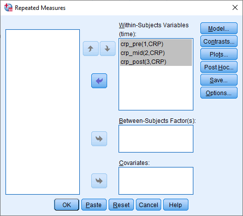
- Transfer crp_pre, crp_mid and crp_post into the "_?_(1,CRP)", "_?_(2,CRP)" and "_?_(3,CRP)" placeholders respectively in the Within-Subjects Variables (time): box, by highlighting all the variables in the left-hand box (by clicking on them whilst holding down the shift-key), and then clicking on the top button. You will end up with the following screen:
Published with written permission from SPSS Statistics, IBM Corporation.
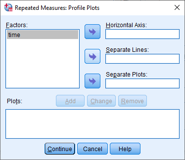
- Click on the button. You will be presented with the Repeated Measures: Profile Plots dialogue box, as shown below:
Published with written permission from SPSS Statistics, IBM Corporation.
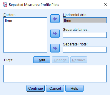
- Transfer the within-subjects factor, time, from the Factors: box into the Horizontal Axis: box by clicking on the top button. You will end up with the following screen:
Published with written permission from SPSS Statistics, IBM Corporation.
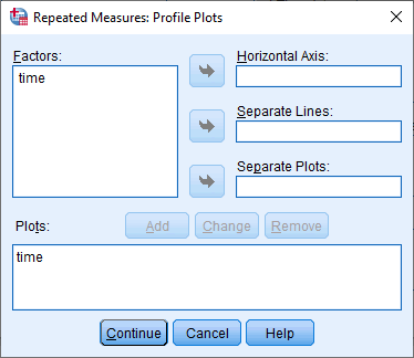
- Click on the button. This will transfer "time" from to the Plots: box, as shown below:
Published with written permission from SPSS Statistics, IBM Corporation.
- Click on the button and you will be returned to the Repeated Measures dialogue box.
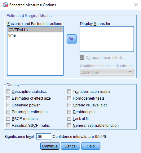
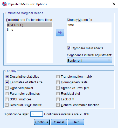
- Click on the button and you will be presented with the Repeated Measures: Options dialogue box, as shown below:
Published with written permission from SPSS Statistics, IBM Corporation.
- Transfer time from the Factor(s) and Factor Interactions: box to the Display Means for: box using the button. This will activate the Compare main effects checkbox (i.e., it will no longer be greyed out). Tick this checkbox and select from the drop-down menu under Confidence interval adjustment:. Next, in the –Display– area, tick the Descriptive statistics and Estimates of effect size checkboxes. You will be presented with the following screen:
Published with written permission from SPSS Statistics, IBM Corporation.
- Click on the button and you will be returned to the Repeated Measures dialogue box.
- Click on the button. This will generate the output.