Independent t-test for two samples
Introduction
The independent t-test, also called the two sample t-test, independent-samples t-test or student's t-test, is an inferential statistical test that determines whether there is a statistically significant difference between the means in two unrelated groups.
Null and alternative hypotheses for the independent t-test
The null hypothesis for the independent t-test is that the population means from the two unrelated groups are equal:
H0: u1 = u2
In most cases, we are looking to see if we can show that we can reject the null hypothesis and accept the alternative hypothesis, which is that the population means are not equal:
HA: u1 ≠ u2
To do this, we need to set a significance level (also called alpha) that allows us to either reject or accept the alternative hypothesis. Most commonly, this value is set at 0.05.
What do you need to run an independent t-test?
In order to run an independent t-test, you need the following:
- One independent, categorical variable that has two levels/groups.
- One continuous dependent variable.
Unrelated groups
Unrelated groups, also called unpaired groups or independent groups, are groups in which the cases (e.g., participants) in each group are different. Often we are investigating differences in individuals, which means that when comparing two groups, an individual in one group cannot also be a member of the other group and vice versa. An example would be gender - an individual would have to be classified as either male or female – not both.
Assumption of normality of the dependent variable
The independent t-test requires that the dependent variable is approximately normally distributed within each group.
Note: Technically, it is the residuals that need to be normally distributed, but for an independent t-test, both will give you the same result.
You can test for this using a number of different tests, but the Shapiro-Wilks test of normality or a graphical method, such as a Q-Q Plot, are very common. You can run these tests using SPSS Statistics, the procedure for which can be found in our Testing for Normality guide. However, the t-test is described as a robust test with respect to the assumption of normality. This means that some deviation away from normality does not have a large influence on Type I error rates. The exception to this is if the ratio of the smallest to largest group size is greater than 1.5 (largest compared to smallest).
What to do when you violate the normality assumption
If you find that either one or both of your group's data is not approximately normally distributed and groups sizes differ greatly, you have two options: (1) transform your data so that the data becomes normally distributed (to do this in SPSS Statistics see our guide on Transforming Data), or (2) run the Mann-Whitney U test which is a non-parametric test that does not require the assumption of normality (to run this test in SPSS Statistics see our guide on the Mann-Whitney U Test).
Assumption of homogeneity of variance
The independent t-test assumes the variances of the two groups you are measuring are equal in the population. If your variances are unequal, this can affect the Type I error rate. The assumption of homogeneity of variance can be tested using Levene's Test of Equality of Variances, which is produced in SPSS Statistics when running the independent t-test procedure. If you have run Levene's Test of Equality of Variances in SPSS Statistics, you will get a result similar to that below:
This test for homogeneity of variance provides an F-statistic and a significance value (p-value). We are primarily concerned with the significance value – if it is greater than 0.05 (i.e., p > .05), our group variances can be treated as equal. However, if p < 0.05, we have unequal variances and we have violated the assumption of homogeneity of variances.
Overcoming a violation of the assumption of homogeneity of variance
If the Levene's Test for Equality of Variances is statistically significant, which indicates that the group variances are unequal in the population, you can correct for this violation by not using the pooled estimate for the error term for the t-statistic, but instead using an adjustment to the degrees of freedom using the Welch-Satterthwaite method. In all reality, you will probably never have heard of these adjustments because SPSS Statistics hides this information and simply labels the two options as "Equal variances assumed" and "Equal variances not assumed" without explicitly stating the underlying tests used. However, you can see the evidence of these tests as below:
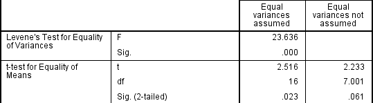
From the result of Levene's Test for Equality of Variances, we can reject the null hypothesis that there is no difference in the variances between the groups and accept the alternative hypothesis that there is a statistically significant difference in the variances between groups. The effect of not being able to assume equal variances is evident in the final column of the above figure where we see a reduction in the value of the t-statistic and a large reduction in the degrees of freedom (df). This has the effect of increasing the p-value above the critical significance level of 0.05. In this case, we therefore do not accept the alternative hypothesis and accept that there are no statistically significant differences between means. This would not have been our conclusion had we not tested for homogeneity of variances.
Reporting the result of an independent t-test
When reporting the result of an independent t-test, you need to include the t-statistic value, the degrees of freedom (df) and the significance value of the test (p-value). The format of the test result is: t(df) = t-statistic, p = significance value. Therefore, for the example above, you could report the result as t(7.001) = 2.233, p = 0.061.
Fully reporting your results
In order to provide enough information for readers to fully understand the results when you have run an independent t-test, you should include the result of normality tests, Levene's Equality of Variances test, the two group means and standard deviations, the actual t-test result and the direction of the difference (if any). In addition, you might also wish to include the difference between the groups along with a 95% confidence interval. For example:
Inspection of Q-Q Plots revealed that cholesterol concentration was normally distributed for both groups and that there was homogeneity of variance as assessed by Levene's Test for Equality of Variances. Therefore, an independent t-test was run on the data with a 95% confidence interval (CI) for the mean difference. It was found that after the two interventions, cholesterol concentrations in the dietary group (6.15 ± 0.52 mmol/L) were significantly higher than the exercise group (5.80 ± 0.38 mmol/L) (t(38) = 2.470, p = 0.018) with a difference of 0.35 (95% CI, 0.06 to 0.64) mmol/L.
To know how to run an independent t-test in SPSS Statistics, see our SPSS Statistics Independent-Samples T-Test guide. Alternatively, you can carry out an independent-samples t-test using Excel, R and RStudio.