One-way repeated measures MANOVA in SPSS Statistics
Introduction
A one-way repeated measures multivariate analysis of variance (i.e., the one-way repeated measures MANOVA), also referred to as a doubly multivariate MANOVA, is used to determine whether there are any differences in multiple dependent variables over time or between treatments, where participants have been measured at all time points or taken part in all treatments. To learn more about these two types of study design where the one-way repeated measures MANOVA is commonly used (i.e., examining "differences over time" and "differences between treatments"), see the examples below:
Note: The one-way repeated measures MANOVA can be thought of as an extension to the one-way repeated measures ANOVA, which is used when you only have one dependent variable or are interested in analysing only one dependent variable at a time, or as the within-subjects (i.e., repeated measures) version of the between-subjects one-way MANOVA, which is used when you are interested in differences between groups that are independent/unrelated rather than groups that are related.
- Differences over TIME
- Differences between TREATMENTS
Imagine that a broadband provider wants to determine whether introducing a new bonus scheme for its sales staff will increase their levels of organisational commitment, where increased organisational commitment generally results in employees staying at an organisation longer and being relatively more productive. Therefore, 30 sales staff are randomly selected to take part in a study where the new bonus scheme is applied to their employment contract. All other things being equal, management at the broadband provider consider the new bonus scheme to be more generous overall, and hope this will increase levels of organisational commitment.
The organisational commitment of the 30 sales staff is measured at three time points: (1) just before the new bonus scheme is introduced; (2) one month after the new bonus scheme is introduced, when the sales staff will receive their first bonuses based on their sales results; and (3) six months after the new bonus scheme is introduced, when sales staff receive their bi-annual reviews. These three time points are designed to allow management at the broadband provider to assess how the new bonus scheme might affect organisational commitment amongst sales staff in the short- and medium-term. At each of these three time points – "pre-bonus", "short-term review" (at Month 1) and "medium-term review" (at Month 6) – three types of organisational commitment are measured using a questionnaire, known as "affective commitment", "continuance commitment" and normative commitment", which each assess different aspects of organisational commitment and are seen a good measures of an employee's overall organisational commitment. The questionnaire provides three scores for each of the 30 sales staff: one score showing their "affective commitment", one score showing their "continuance commitment", and another score showing their "normative commitment".
Therefore, in this experiment "organisational commitment" is assessed using three dependent variables, "affective commitment", "continuance commitment" and normative commitment", and the independent variable is "time", with three related groups: "pre-bonus", "short-term review" and "medium-term review". The three groups are related because all 30 sales staff were measured in terms of each dependent variable at all three time points, so each employee has nine scores: one for each of the three dependent variables at each time point (i.e., 3 x 3 = 9).
The broadband provider analyses the data collected using a one-way repeated measures MANOVA to determine whether there is a statistically significant difference in organisational commitment – measured in terms of affective commitment, continuance commitment and normative commitment combined – over the three time points: pre-bonus, short-term review and medium-term review.
Imagine that large chain of opticians want to determine whether a new type of lens used in glasses improves patients' vision. Therefore, 80 patients are randomly selected to take part in a study where they are asked to wear glasses with two different types of lens: (a) the "standard" lens that they sell; and (b) the "new" lens they are considering whether to introduce. When wearing each of the two types of lens, the 80 participants complete a "visual acuity test" and a "depth perception test", which together are used to assess the performance of each lens in improving patients' vision.
Therefore, in this experiment "lens performance" is assessed using two dependent variables, "visual acuity" and "depth perception", and the independent variable is "lens type", with two related groups: the "standard lens" and the "new lens". The two groups are related because all 80 participants were tested using both lenses, so each participant has four scores: a "visual acuity" score and a "depth perception" score for the "standard" lens and the "new" lens (i.e., 2 x 2 = 4).
The optician analyses the data collected using a one-way repeated measures MANOVA to determine whether there is a statistically significant difference in lens performance – measured in terms of visual acuity and depth perception combined – based on whether the standard lens or new lens was used.
If a one-way repeated measures MANOVA is statistically significant, this would suggest that there is a difference in the combined dependent variables between the two or more related groups. Taking the first example above, a statistically significant one-way repeated measures MANOVA would suggest that there was a difference in the three combined types of organisational commitment – that is, the three dependent variables: "affective commitment", "continuance commitment" and normative commitment" – between the "pre-bonus", "short-term review" and "medium-term review" time points (i.e., before, 1 month after and 6 months after the new bonus scheme was introduced), which represent the three related groups.
However, the one-way repeated measures MANOVA is an omnibus test, which means that it cannot tell us where the differences are when you have three or more related groups. For example, it cannot tell us that these three combined types of organisational commitment were different at the "short-term review" time point compared to the "pre-bonus" time point. Similarly, the one-way repeated measures MANOVA cannot tell us that there was a difference in the combined organisational commitment score between the "short-term review" and "medium-term review". It can only tell us that at least two related groups (i.e., time points) were different.
Since you may have three, four, five or more time points (or treatments) in your study design, determining which of these related groups differ from each other is important. Therefore, you can determine where these differences are by carrying out a follow-up analysis (also known as post hoc testing). If you are interested in understanding which related groups are different at the multivariate level (i.e., where the differences are between the combined dependent variables), you can consider multivariate contrasts. However, if you are interested in understanding which related groups are different at the univariate level (i.e., where the differences are between each dependent variable separately), you can consider a univariate analysis. Alternatively, if you are interested in how the combined dependent variables change over time between each related group (e.g., how the combined scores of the dependent variables change from the "pre-bonus", to the "short-term review", and then to the "medium-term review"), you can assess whether there are any polynomial trends.
Note: If you would like us to expand this section to explain these three different types of follow-up analysis (i.e., multivariate contrasts, univariate analysis and polynomial trends), please contact us.
In this "quick start" guide, we show you how to carry out a one-way repeated measures MANOVA using SPSS Statistics and which table you need to use to determine whether you have a statistically significant result. However, before running the one-way repeated measures MANOVA you need to understand the different assumptions that your data must meet in order for a one-way repeated measures MANOVA to give you a valid result. We discuss these assumptions next.
SPSS Statistics
Assumptions of a one-way repeated measures MANOVA
When you choose to analyse your data using a one-way repeated measures MANOVA, part of the process involves checking to make sure that the data you want to analyse can actually be analysed using a one-way repeated measures MANOVA. You need to do this because it is only appropriate to use a one-way repeated measures MANOVA if your data passes seven assumptions that are required for a one-way repeated measures MANOVA to give you a valid result. Do not be surprised if, when analysing your own data using SPSS Statistics, one or more of these assumptions is violated (i.e., is not met). This is not uncommon when working with real-world data. However, even when your data fails certain assumptions, there is often a solution to overcome this.
In practice, checking for these seven assumptions adds some more time to your analysis, requiring you to work through additional procedures in SPSS Statistics when performing your analysis, as well as thinking a little bit more about your data. These seven assumptions are presented below:
- Assumption #1: Your two or more dependent variables should be measured at the interval or ratio level (i.e., they are continuous variables). Examples of continuous variables include revision time (measured in hours), intelligence (measured using IQ score), exam performance (measured from 0 to 100), weight (measured in kg), and so forth. You can learn more about interval and ratio variables in our article: Types of Variable.
- Assumption #2: Your independent variable should consist of two or more categorical, related groups. Groups can be considered to be related when a participant is measured at all time points or receives all treatments. Alternatively, participants can be matched (e.g., twins, family members). Whilst groups should be related, participants should be independent, such that one participant should not be able to influence the scores of another participant.
- Assumption #3: You should have an adequate sample size. Although the larger your sample size the better, for a one-way repeated measures MANOVA to run, you need to have more cases (e.g., participants) in each related group than the number of dependent variables you are analysing. For example, if you had six dependent variables where participants were measured over five time points (i.e., you have five related groups), there must be at least six participants in each of the five related groups for the one-way repeated measures MANOVA to run.
- Assumption #4: There should be no univariate or multivariate outliers. First, there should be no (univariate) outliers in each related group of the independent variable for any of the dependent variables. This is a similar assumption to the one-way repeated measures ANOVA, but for each dependent variable that you have in your one-way repeated measures MANOVA analysis. Univariate outliers are often just called outliers and are the same type of outliers you will have come across if you have ever conducted t-tests or ANOVAs. We refer to them as univariate in this guide to distinguish them from multivariate outliers, which are cases (e.g., participants) which have an unusual combination of scores on the dependent variables.
- Assumption #5: There should be multivariate normality. Unfortunately, multivariate normality is a particularly tricky assumption to test for and cannot be directly tested in SPSS Statistics. Instead, normality of each of the dependent variables for each of the related groups of the independent variable is often used in its place as a best 'guess' as to whether there is multivariate normality. You can test for normality in SPSS Statistics using numerical methods such as the Shapiro-Wilk test of normality and graphical methods such as histograms and Normal Q-Q plots.
- Assumption #6: There should be a linear relationship between each pair of dependent variables for each related group of the independent variable. If the variables are not linearly related, the power of the test is reduced. You can test for this assumption by plotting a scatterplot matrix for each related group of the independent variable.
- Assumption #7: There should be no multicollinearity. Ideally, you want your dependent variables to be moderately correlated with each other. If the correlations are low, you might be better off running separate one-way repeated measures ANOVAs, and if the correlations are too high (generally considered greater than 0.9), you could have multicollinearity. This is problematic for the one-way repeated measures MANOVA and needs to be screened out.
You can check assumptions #4 through #7 using SPSS Statistics. Before doing this, you should make sure that your data meets assumptions #1 through #3, although you don't need SPSS Statistics to do this. Just remember that if you do not run the statistical tests on these assumptions correctly, the results you get when running a one-way repeated measures MANOVA might not be valid.
Note: When we launch our premium one-way repeated measures MANOVA guide, we will show you how to check assumptions #4 through #7 in SPSS Statistics to make sure that your data has passed these assumptions, and if it fails any, explain what you can do in order to continue with your analysis. If you would like us to email you when this guide becomes available, please contact us.
In the section, Procedure, we illustrate the SPSS Statistics procedure to perform a one-way repeated measures MANOVA assuming that no assumptions have been violated. First, we set out the example we use to explain the one-way repeated measures MANOVA procedure in SPSS Statistics.
SPSS Statistics
Example used in this guide
In this fictitious study, a researcher would like to know whether only five minutes of extremely high-intensity exercise per day can improve "cardiovascular health", which was being determined using three biomarkers: "cholesterol concentration", "systolic blood pressure" and "glucose concentration".
Therefore, the researcher recruited 30 participants and asked each participant to carry out a 6-month exercise training programme, which consisted of only five minutes of extremely high-intensity exercise per day. The introduction of an exercise training programme can be thought of as an intervention that the researcher is using to understand whether this extremely high-intensity exercise programme results in a change in cardiovascular health, where a lower score in the three biomarkers – "cholesterol concentration", "systolic blood pressure" and "glucose concentration" – would reflect better cardiovascular health and a higher score would reflect poorer cardiovascular health (i.e., all other things being equal and "generally speaking", higher levels of cholesterol concentration, systolic blood pressure and glucose concentration are associated with poorer cardiovascular health).
As such, the researcher records the 30 participants' levels of cholesterol concentration, systolic blood pressure and glucose concentration at three time points: "pre-intervention" (i.e., just before the exercise programme starts), "mid-intervention" (i.e., 3 months after the exercise programme started), and "post-intervention" (i.e., 6 months after the exercise programme started, when the experiment ends).
In order to determine whether cardiovascular health has improved during the intervention, the researcher runs a one-way repeated measures MANOVA to determine the change in the three biomarkers collectively over time.
Therefore, in this fictitious study the three continuous dependent variables are cholesterol (i.e., representing "cholesterol concentration"), bps (i.e., representing "systolic blood pressure") and glucose (i.e., representing "glucose concentration"). The independent variable is time, which consists of three related groups – "pre", "mid" and "post" – which reflect the three time points when the three dependent variables are measured for each of the 30 participants. When setting up your data in SPSS Statistics, the data for these dependent variables and related groups must be combined. Therefore, since we have three dependent variables and three related groups, we created the following nine variables in SPSS Statistics (i.e., 3 x 3 = 9): pre_chol, mid_chol and post_chol (i.e., for the three related groups of cholesterol), pre_sbp, mid_sbp and post_sbp (i.e., for the three related groups of sbp), and pre_gluc, mid_gluc and post_gluc (i.e., for the three related groups of glucose). In the next section, we show you how to run a one-way repeated measures MANOVA in SPSS Statistics using these nine variables.
SPSS Statistics
SPSS Statistics procedure to carry out a one-way repeated measures MANOVA
The nine steps below show you how to analyse your data using a one-way repeated measures MANOVA in SPSS Statistics when the seven assumptions in the previous section, Assumptions, have not been violated. At the end of these nine steps, we show you how to interpret the results from this test, as well as explain the additional analyses you will need to carry out in SPSS Statistics to follow-up the results from a one-way repeated measures MANOVA.
Note: The procedure that follows is identical for SPSS Statistics versions 18 to 30, as well as the subscription version of SPSS Statistics, with version 30 and the subscription version being the latest versions of SPSS Statistics. However, in version 27 and the subscription version, SPSS Statistics introduced a new look to their interface called "SPSS Light", replacing the previous look for versions 26 and earlier versions, which was called "SPSS Standard". Therefore, if you have SPSS Statistics versions 27 to 30 (or the subscription version of SPSS Statistics), the images that follow will be light grey rather than blue. However, the procedure is identical.
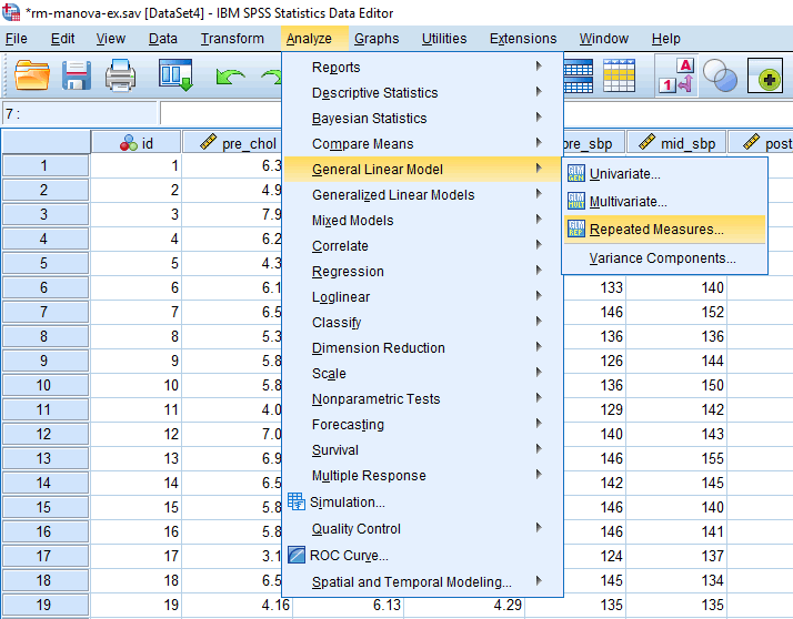
- Click Analyze > General Linear Model > Repeated Measures... on the top menu, as shown below:

Published with written permission from SPSS Statistics, IBM Corporation.
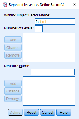
You will be presented with the Repeated Measures Define Factor(s) dialogue box:

Published with written permission from SPSS Statistics, IBM Corporation.
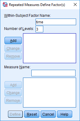
- Enter the name of your independent variable (e.g., "time", to represent our independent variable, time) into the Within-subject Factor Name: box, followed by the number of related groups of your independent variable (e.g., "3", to reflect our three related groups: "pre", "mid" and "post") into the Number of Levels: box, as shown below:

Published with written permission from SPSS Statistics, IBM Corporation.
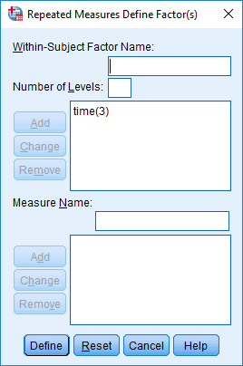
- Click on the top
 button. This should transfer the name of your independent variable and the number of related groups for that independent variable (e.g., "time(3)") into the box immediately below. You should end up with a screen similar to the one below, but with the name of your independent variable and the number of related groups for that independent variable added into the box:

Published with written permission from SPSS Statistics, IBM Corporation.
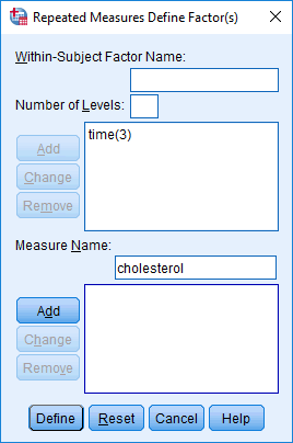
- Enter the name of one of your dependent variables (e.g., "cholesterol", to represent the dependent variable, cholesterol) into the Measure Name: box, as shown below:

Published with written permission from SPSS Statistics, IBM Corporation.
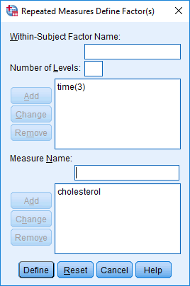
- Click on the bottom
 button. This should transfer the name of the dependent variable (e.g., "cholesterol") into the box immediately below. You should end up with a screen similar to the one below, but with the name of one of your dependent variables added into the box:

Published with written permission from SPSS Statistics, IBM Corporation.
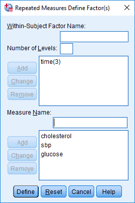
- Repeat Step 5 and Step 6 above, but for your remaining dependent variables (e.g., "sbp" and "glucose", to represent our two remaining dependent variables, sbp and glucose, respectively). You should end up with a screen similar to the one below, but with the name of all of your dependent variables added into the box:

Published with written permission from SPSS Statistics, IBM Corporation.
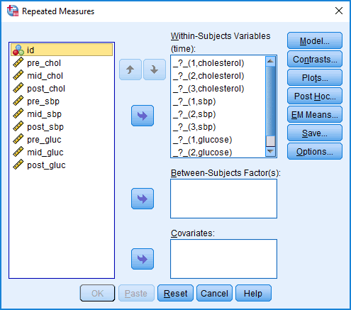
- Click on the
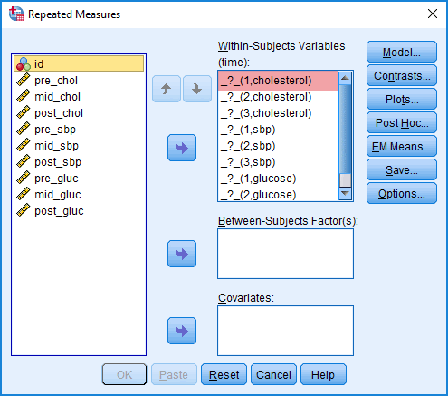
 button. You will be presented with the Repeated Measures dialogue box, as shown below:

Published with written permission from SPSS Statistics, IBM Corporation.
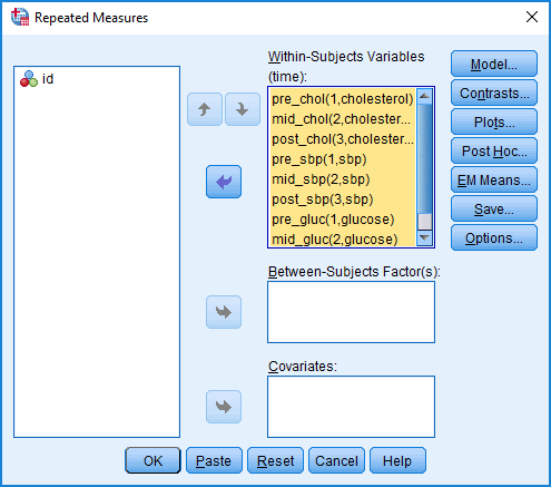
- Transfer the variables representing the combined dependent variables and related groups into the Within-Subjects Variables (time): box based on the combination of related groups and dependent variables shown in the Within-Subjects Variables (time): box. In our example, there are nine variables to transfer – pre_chol through to post_gluc – representing the three time points – "pre", "mid" and "post" – and three dependent variables: cholesterol, sbp and glucose, as shown below:

Published with written permission from SPSS Statistics, IBM Corporation.
Explanation: You need to make sure that the correct variables are transferred into the Within-Subjects Variables (time): box. Therefore, look again at the first placeholder for one of our variables in the Within-Subjects Variables (time): box from Step 8, as highlighted below:

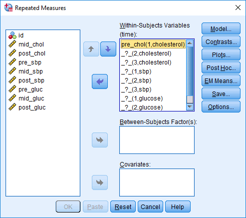
This placeholder is called "_?_(1,cholesterol)". This tells us that we need to enter the variable that represents the first related group (i.e., "1"), which is "pre" in our example, for the dependent variable, cholesterol (i.e., "cholesterol"). Therefore, we transferred the variable, pre_chol, into the first placeholder of the Within-Subjects Variables (time): box, as highlighted below:

The name of the first placeholder in the Within-Subjects Variables (time): box has now changed from "_?_(1,cholesterol)" to "pre_chol(1,cholesterol)". You now have to repeat this process for all of your variables (i.e., for the 8 remaining variables in our example).
- Click on the
 button. This will generate the results for the one-way repeated measures MANOVA.
SPSS Statistics
Interpreting the results of a one-way repeated measures MANOVA
SPSS Statistics produces many different tables when you run a one-way repeated measures MANOVA analysis. In this section, we show you how to determine whether your one-way repeated measures MANOVA is statistically significant. If a one-way repeated measures MANOVA is statistically significant, this would suggest that there is a difference in the combined dependent variables between the two or more related groups.
Therefore, in our example a statistically significant one-way repeated measures MANOVA would suggest that there was a difference in the three combined biomarkers – that is, our three dependent variables: cholesterol, sbp and glucose – between the "pre", "mid" and "post-intervention" time points (i.e., before the exercise intervention, 3 months after the exercise intervention started and at the end of the exercise intervention), which represent our three related groups.
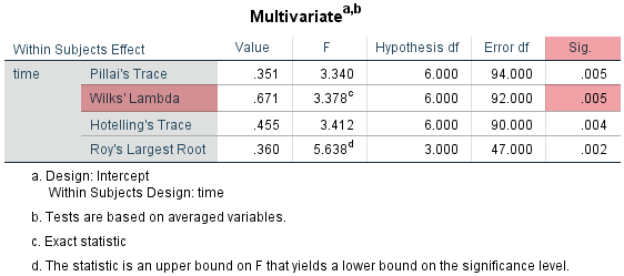
You can determine whether the one-way repeated measures MANOVA is statistically significant by consulting the "Sig." column along the "Wilks' Lambda" row of the Multivariate Tests table, as highlighted below:

Published with written permission from SPSS Statistics, IBM Corporation.
The "Sig." column presents the significance value (i.e., p-value) of the one-way repeated measures MANOVA. If p < .05 (i.e., if p is less than .05), the one-way repeated measures MANOVA is statistically significant. Alternatively, if p > .05 (i.e., if p is greater than .05), the one-way repeated measures MANOVA is not statistically significant.
You can see from the highlighted row under the "Sig." column above (along the "Wilks' Lambda" row) that p = .005. Since .005 is less than .05 (i.e., it satisfies p < .05), the one-way repeated measures MANOVA is statistically significant. In other words, there is a difference in the three combined biomarkers – cholesterol, sbp and glucose – over time – pre-, mid- and post-intervention – when an extremely high-intensity exercise programme is introduced.
Note: Whilst there is a statistically significant difference, without a control group who did not exercise, we would not conclude that the extremely high-intensity exercise programme caused the change in these three biomarkers, but perhaps suggest that is might have (i.e., a result that would be worth further investigation, perhaps by adding a control group).
As discussed in the Introduction, if the one-way repeated measures MANOVA is statistically significant, you can follow-up this result to determine which of the two or more related groups differed in terms of the combined dependent variables. For example, our results suggest that there is a difference in the three combined biomarkers – cholesterol, sbp and glucose – over time – pre-, mid- and post-intervention – when an extremely high-intensity exercise programme is introduced. However, the one-way repeated measures MANOVA is an omnibus test, which means that it cannot tell us where the differences are between our three related groups. For example, it cannot tell us that these three combined biomarkers were different at the "mid-intervention" time point compared to the "pre-intervention" time point. Similarly, the one-way repeated measures MANOVA cannot tell us that there was a difference in the score of the three combined biomarkers between the "med-intervention" and "post-intervention" time points. It can only tell us that at least two related groups (i.e., time points) were different.
Note: If you are carrying out a one-way repeated measures MANOVA with only two related groups, the results will tell you which groups differed in terms of the combined dependent variables. After all, you are only comparing two related groups, so there is only one pairwise comparison (i.e., "Group A versus Group B"). For example, think back to our example of study designs that look at "differences between treatments" in the Introduction, where the researcher was interested in the differences in "lens performance" between a "standard" lens and a "new" lens (i.e., where the two related groups are the "standard" lens and "new" lens). Since there are only two related groups, if the one-way repeated measures MANOVA is statistically significant, it will tell us that there is a difference between these two related groups (i.e., because these are the only two related groups you are comparing). However, when you have three or more related groups, there are multiple pairwise comparisons. For example, with three related groups there are three pairwise comparisons (i.e., "Group A versus Group B", "Group A versus Group C", and "Group B versus Group C"). Therefore, when you have three or more related groups, the one-way repeated measures MANOVA cannot tell us which of the pairwise comparisons are different. It can only tell us that at least one pairwise comparison is different.
Since you may have three, four, five or more time points (or treatments) in your study design, determining which of these related groups differ from each other is important. Therefore, you can determine where these differences are by carrying out a follow-up analysis (also known as post hoc testing). If you are interested in understanding which related groups are different at the multivariate level (i.e., where the differences are between the combined dependent variables), you can consider multivariate contrasts. However, if you are interested in understanding which related groups are different at the univariate level (i.e., where the differences are between each dependent variable separately), you can consider a univariate analysis. Alternatively, if you are interested in how the combined dependent variables change over time between each related group (e.g., how the combined scores of the dependent variables change from the "pre-bonus", to the "short-term review", and then to the "medium-term review"), you can assess whether there are any polynomial trends.
Which of these three types of follow-up analysis (i.e., multivariate contrasts, univariate analysis and polynomial trends) you should carry out will depend on your goals (i.e., research questions and/or hypotheses) because they will tell you different things about your data. Therefore, if you would like us to expand this section to explain more about these three different types of follow-up analysis, please contact us.
SPSS Statistics
Short Bibliography
Keppel, G., & Wicken, T. D. (2004). Design and analysis: A researcher's handbook (4th ed.). Upper Saddle River, NJ: Prentice Hall.
Keselman, H. J., Rogan, J. C., Mendoza, J. I., & Breen, I. I. (1980). Testing the validity conditions of repeated measures F tests. Psychological Bulletin, 87, 479-487.
Maxwell, S. E., & Delaney, H. D. (2004). Designing experiments and analyzing data: A model comparison perspective (2nd ed.). Mahwah, NJ: Lawrence Erlbaum.
Norušis, M. J. (2012). IBM SPSS Statistics 19 advanced statistical procedures companion. Upper Saddle River, NJ: Prentice Hall.
Rogan, J. C., Keselman, H. J., & Mendoza, J. I. (1979). Analysis of repeated measurements. British Journal of Mathematical and Statistical Psychology, 32, 269-286.
Weinfurt, K. P. (1995). Multivariate analysis of variance. In Grimm, L. G. & P. R. Yarnold (Ed.), Reading and understanding multivariate statistics (pp 245-276). Washington, DC: American Psychological Association.

