Independent-samples t-test using R, Excel and RStudio (page 4)

On the previous page you learnt how to carry out an independent-samples t-test, including useful descriptive statistics. On this page you will learn how to interpret the results for the independent-samples t-test, as well as descriptive statistics that include the group means, standard deviations, sample sizes, and the mean difference. Finally, we explain how you can report your results in-text and using a graph. Therefore, start by learning how to interpret the independent-samples t-test results in the next section.

R and RStudio

Interpreting the independent-samples t-test results

After carrying out the t.test, descriptives and mean_difference procedures using R in the previous two sections, RStudio will display a set of results that contain all the information you need to interpret and report the results from an independent-samples t-test.

In this section, we explain how to interpret these results, assuming your data has already met (i.e., "passed") the assumptions of no significant outliers (Assumption #4), a dependent variable that is approximately normally distributed for each category of your independent variable (Assumption #5), and homogeneity of variances (Assumption #6), as discussed in the Assumptions section earlier. For example, if our data did not meet any of these three assumptions, the results for the independent-samples t-test discussed in this section might be invalid/inaccurate and it is possible that the conclusions would also be incorrect. Therefore, it is extremely important that you first check whether your data meets these three assumptions before interpreting the results from the independent-samples t-test. However, in this "quick start" guide, we simply show you how to interpret the results from the independent-samples t-test, assuming your data has already met these important assumptions.

Descriptive statistics

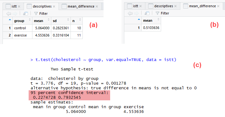
To start your analysis, look at the useful descriptive statistics that were produced when you ran: (a) the descriptives; (b) the mean_difference; and (c) t.test procedures earlier, as shown side-by-side below:

The descriptives output on the left above presents the mean (i.e., under the column), standard deviation (i.e., under the column) and sample size (i.e., under the column) for the "control group" and "exercise group" (i.e., along rows and respectively). The mean_difference output on the right above presents the mean difference (i.e., under the column). The highlighted t.test output at the bottom above presents the 95% confidence interval (CI) of the mean difference.

The results show that the mean cholesterol concentration in the "control group" was 5.06 mmol/L (to 2 decimal places) with a standard deviation of 0.28 mmol/L. There were 10 participants in the control group. In the "exercise group", mean cholesterol concentration was 4.55 mmol/L with a standard deviation of 0.33 mmol/L. There were 11 participants in the exercise group. Therefore, there was a mean difference of 0.51 mmol/L between the control group and exercise group, with cholesterol concentration being 0.51 mmol/L higher in the control group (i.e., 5.064 – 4.554 = 0.51 mmol/L). The 95% confidence interval (CI) of the mean difference was from 0.23 mmol/L (for the lower bound value; to 2 decimal places) to 0.79 mmol/L (for the upper bound value).

Therefore, in our sample of 21 participants it appears that the sedentary people who underwent a 6-month exercise programme had lower cholesterol concentration at the end of this programme compared to the control group who underwent their usual everyday activities for 6 months. With a mean difference of 0.51 mmol/L, and 95% confidence interval (CI) of the mean difference of 0.23 mmol/L to 0.79 mmol/L, this may be of practical significance, meaning that from a health perspective, the difference in cholesterol concentration between the groups may be important or at least interesting.

You can also determine whether the mean difference between the two groups is statistically significant; that is, based on our sample of 21 participants, whether there is a mean difference in cholesterol concentration between the exercise group and control group in the population from which our sample was drawn. This is discussed in the next section.

Independent-samples t-test

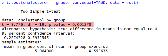
The independent-samples t-test results were produced when you ran the t.test() function earlier. The t.test output presents the obtained t-value (t), the degrees of freedom (df), and the statistical significance value (p-value) of the independent-samples t-test, as highlighted below:

Note: The t.test output also presents the 95% confidence interval (CI) of the mean difference (lower and upper bounds), and the mean of the two groups. However, it does not include the mean difference, standard deviation or sample size of the two groups, which is why we showed you how to carry out the descriptives and mean_difference procedures earlier.

From the t.test output above, the obtained t-value (t) is 3.78 (to 2 decimal places) and the degrees of freedom (df) are 19 (i.e., for an independent-samples t-test the degrees of freedom are equal to the sample size minus 2, so in our example, 21 – 2 = 19). The statistical significance (p-value) of the independent-samples t-test is 0.001.

The p-value is used to determine if there is a statistically significant difference in the mean score of the dependent variable between the two independent groups. If p < .05 (i.e., if p is less than .05), there is a statistically significant difference in mean cholesterol concentration between the control group and exercise group. If p > .05 (i.e., if p is greater than .05), there is not a statistically significant difference in mean cholesterol concentration between the control group and exercise group. Since p = .001 in our example, there is a statistically significant difference in mean cholesterol concentration between the control group and exercise group (i.e., there is a mean difference in the population and not only the sample that was studied).

Effect size for the independent-samples t-test

The independent-samples t-test, as a null hypothesis significance test, informs you whether a mean difference between the two groups exists in the population (i.e., the mean difference is not zero in the population), but it does not inform you of the size of the difference. To try to overcome this limitation, an effect size can be calculated.

There are many different types of effect size, with different types often trying to "capture" the importance of your results in different ways. If you would like us to add a section discussing effect sizes for the independent-samples t-test, please contact us.

In the next section we explain how to report the results of an independent-samples t-test.

R and RStudio

Reporting the results of an independent-samples t-test

When you report the results of an independent-samples t-test, it is good practice to include the following information:

• A. An introduction to the analysis you carried out.
• B. Information about your sample, including the number of participants (n) in each of your two groups. This is useful to understand whether you have a balanced or unbalanced design (i.e., whether there were an equal or unequal number of participants between the two groups), as well as highlighting any missing values.
• C. A statement of whether there was a statistically significant difference between your two groups, including the group means, standard deviations, estimated mean difference, 95% confidence interval (CI) for the mean difference, t-value, degrees of freedom (df), and statistical significance value (i.e., the p-value).
• D. A table of your results if you have conducted more than one independent-samples t-test. Whilst a table can be used when you have only carried out one independent-samples t-test, as in our example, it often makes sense to simply report such results in-text rather than using a table. In contrast, tables are useful when you have a lot more results to report (i.e., when you have run multiple independent-samples t-tests).
• E. A suitable graph to illustrate the means and distribution of scores of the dependent variable in the two groups of your independent variable. The choice of graph can depend on personal preferences, but also the size of your sample.

  Note: Whilst you can present your results in-text, using a table and a graph, many reporting styles do not favour the duplication of results using all three methods. For example, if your results are explained in detail in-text, the use of a table and/or graph may be viewed as an unnecessary duplication. However, if you do not have to work to a specific reporting style, simply make sure that you are fully explaining your results in a way that the reader can understand, irrespective of whether you do this in-text, using a table and/or a graph.

Based on the results from the independent-samples t-test and associated descriptive statistics in the previous section, we could report the results of this fictitious study as follows:

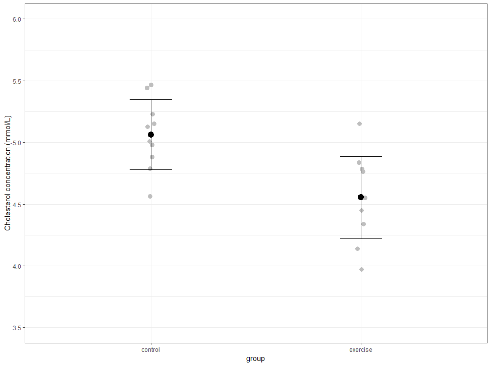
The results from an independent-samples t-test can be illustrated using different types of graph, depending on what you are trying to highlight and the characteristics of your data (e.g., the size of your sample). One such graph is a jittered dot plot with superimposed mean and standard error "error bars", as highlighted below:

A jittered dot plot with superimposed mean and standard error "error bars" shows:

• A. The values for the dependent variable on the y-axis for the two groups displayed on the x-axis. Therefore, in our example, cholesterol concentration is displayed on the y-axis, measured in mmol/L, and the two groups of our independent variable, the "control" group and the "exercise" group are displayed on the x-axis.
• B. The mean score for each group of the independent variable as a bold black dot in the middle of the dot plot.
• C. The spread of scores along the y-axis for each group of the independent variable, where each lighter coloured black/grey dot represents a single case (e.g., participant) in your data set.
• D. The standard error "error bars" (i.e., one above and one below the mean score) for each group of the independent variable, which give you an idea of the variability of the mean.

The information from this jittered dot plot helps to highlight that:

• A. The mean cholesterol concentration was higher in the "control" group who carried on their usual sedentary activities compared to the "exercise" group who undertook a 6-month exercise intervention.
• B. The distribution of cholesterol concentration scores was more clustered around the mean in the "control" group compared to the "exercise" group (i.e., there was less variation in the cholesterol concentration scores amongst participants in the control group).

The jittered dot plot is also useful when discussing outliers and normality, which are two important assumptions of the independent-samples t-test. However, it should be stressed that the jittered dot plot alone would be insufficient to test whether your data has met these assumptions.

Note: This completes our introductory guide to the independent-samples t-test using R (with Excel and RStudio). If you have any comments/feedback about this guide or if you would like us to add other guides to Laerd Statistics, please contact us and let us know how we can help.

R and RStudio

Bibliography

Myers, J. L., Well, A. D., & Lorch, R. F. Jr. (2010). Research design and statistical analysis (3rd ed.). New York, NY: Routledge.

Satterthwaite, F. E. (1946). An approximate distribution of estimates of variance components. Biometrics Bulletin, 2, 110-114.

Sheskin, D. J. (2011). Handbook of parametric and nonparametric statistical procedures (5th ed.). Boca Raton, FL: Chapman & Hall/CRC Press.

Welch, B. L. (1947). The generalization of "Student's" problem when several different population variances are involved. Biometrika, 34(1–2), 28–35.