Independent-samples t-test using R, Excel and RStudio (page 3)

On the previous page you learnt how to set up your data using Excel, R and RStudio, based on the example we use throughout this introductory guide. On this page we show you how to: (a) carry out an independent-samples t-test using the t.test () function; (b) generate useful descriptive statistics including the group means, standard deviations, sample sizes, and the mean difference. Therefore, start by learning how to use the t.test () function to carry out an independent-samples t-test in the next section.

R and RStudio

Running an independent-samples t-test using R in RStudio

The independent-samples t-test is run using R code in RStudio, which you enter into the RStudio Console (i.e., under the tab), as shown below:

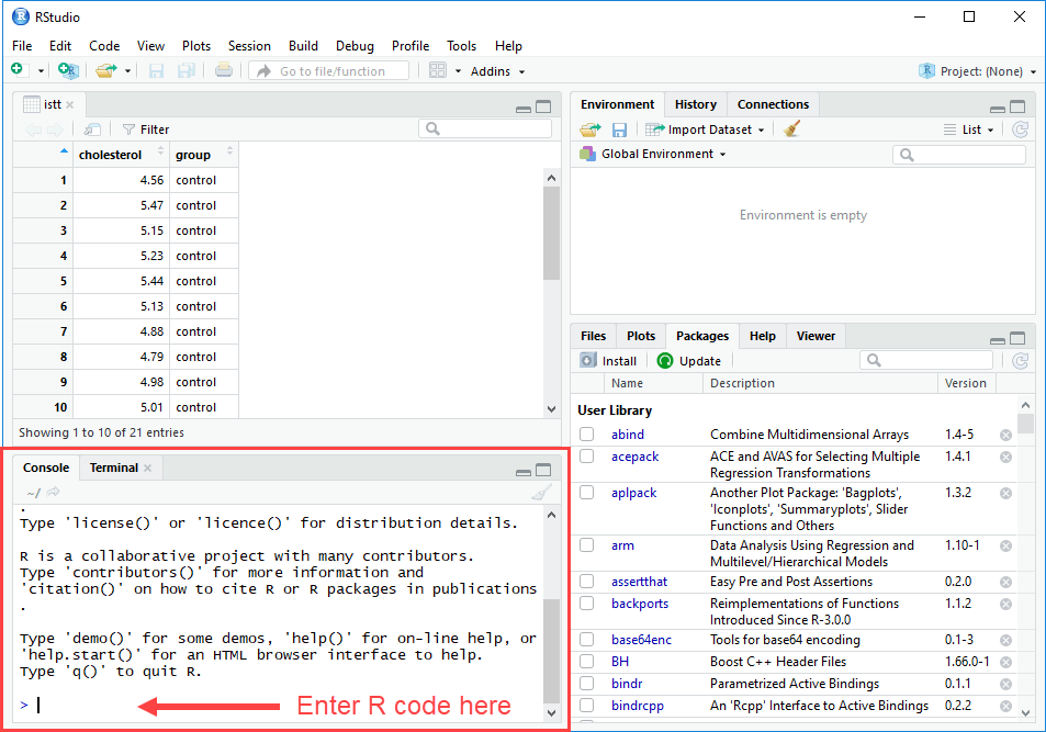
In the three steps that follow we explain how to run an independent-samples t-test using R:

• The code to run an independent-samples t-test using R is as follows:

  t.test (dv ~ iv, var.equal=TRUE, data = dataframe)

  More specifically, this R code has the following meaning:

  t.test (  )	Run a t-test based on the variables and information/options included between the brackets (  ). Enter this R code exactly as shown without making any changes. Note: The t.test () function can be used to run several t-tests, including the one-sample t-test, independent-samples t-test (as demonstrated in this guide), Welch t-test, and paired-samples t-test. Which t-test is run will depend on what variables and options are entered between the brackets (  ).
  dv ~ iv,	Run a t-test using the dv (i.e., dependent variable) and iv (i.e., independent variable) included between the brackets. In other words, replace the words dv and iv with the names of your dependent and independent variables respectively, exactly as you spelt them in Step One in Excel earlier in this guide. Notice that a tilde (~) is entered between the name of the dependent and independent variable. Also notice that a comma (,) is entered at the end of this R code.
  var.equal=TRUE,	Run an independent-samples t-test. This option also assumes that the data has met the assumption of homogeneity of variances, as discussed earlier. Enter this R code exactly as shown without making any changes. Note: This code is only relevant if your data has met this assumption. Again, notice that a comma (,) is entered at the end of this R code.
  data = dataframe	Run an independent-samples t-test on the data that was imported into the dataframe. More specifically, this is telling R where to look for the data of your dependent and independent variables. The R code data = should be entered exactly as shown. However, the word dataframe should be replaced with the name of your dataframe (e.g., istt in our example). Note: If you are unsure what name you gave your dataframe, see the important note in Step 3 of the section: Import your data from Microsoft Excel into RStudio.

• Using the instructions above, we entered the following R code into the RStudio Console (i.e., under the tab):

  t.test (cholesterol ~ group, var.equal=TRUE, data = istt)

  Therefore, the R code above will run an independent-samples t-test assuming that the assumption of homogeneity of variances has been met based on the istt data set that is being used to determine if there is a mean difference between the two groups of our independent variable, group (i.e., the "control" and "exercise" groups of our exercise trial) in terms of the scores of our dependent variable, cholesterol (i.e., the cholesterol of participants, measured in mmol/L).

• Press the Enter/Return key on your keyboard to run the independent-samples t-test. The following output is generated by RStudio in the area, which includes: (a) the R code that you have just run (i.e., in the red rectangle); and (b) the results for the independent-samples t-test (i.e., in the blue rectangle):

  

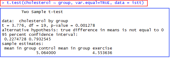
The t.test() function we have just demonstrated provides the minimum results required to understand an independent-samples t-test, such as the t-value, degrees of freedom (df), statistical significance value (i.e., the p-value), 95% confidence interval (CI) of the mean difference, and the mean score for each of your two groups. Each of these statistics will be explained later in the section: Interpreting the independent-samples t-test results. However, there are additional descriptive statistics that are required to get a more complete understanding of your results when running an independent-samples t-test that are not provided by the t.test() function. Therefore, in the next section we explain how to generate these descriptive statistics using R in RStudio.

R and RStudio

Generating descriptive statistics for an independent-samples t-test using R in RStudio

When carrying out an independent-samples t-test, we want to be able to compare the two groups of our independent variable descriptively in terms of the dependent variable. Useful descriptive statistics include the group means, standard deviations, sample sizes, and the mean difference, which is the difference between the two group means. Only the group means are generated by the t.test() function in the previous section. Therefore, the following five steps show you how to generate these descriptive statistics.

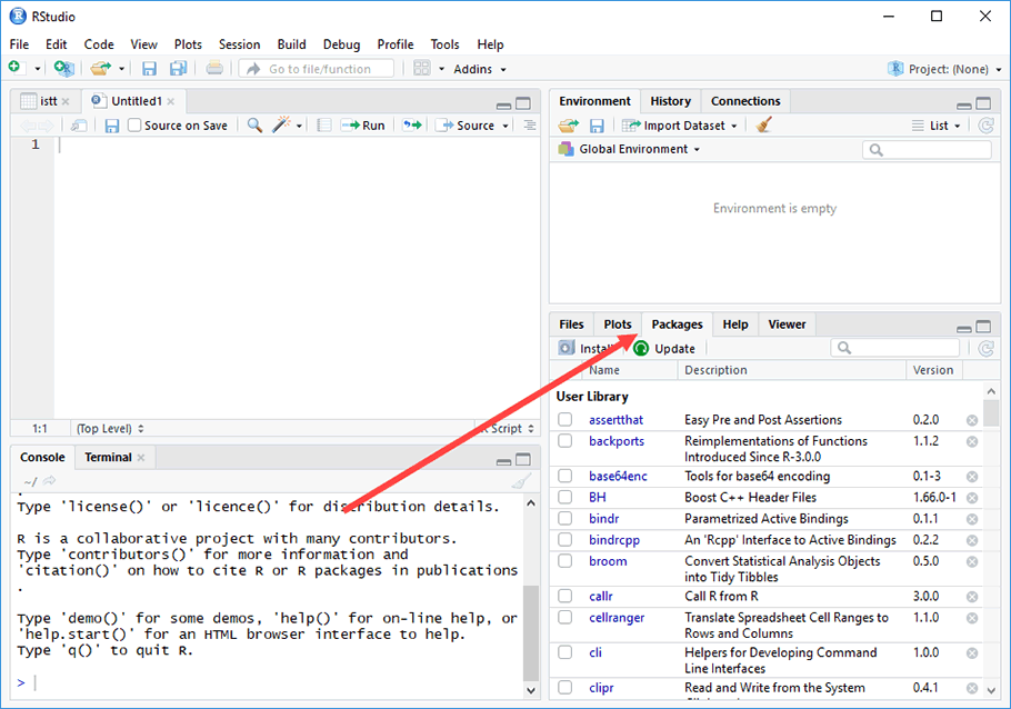
• If not already selected, click on the tab so that the list of R packages is presented, as shown below:

  

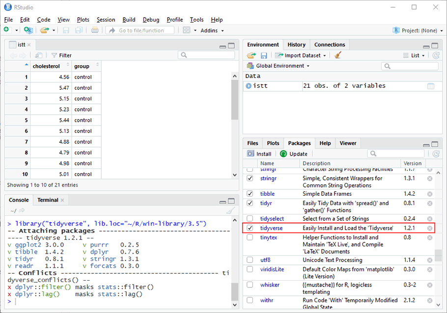
• Select the tidyverse R package from the list of packages, as highlighted below:

  

  Note 1: If you cannot find the tidyverse R package, go back to the section: STEP TWO: Install the tidyverse package into R using RStudio.

  Note 2: When you select the tidyverse R package, the features in this package will become activated, as highlighted in the RStudio Console (i.e., under the tab) above.

• The code to generate the mean, standard deviation and sample size for each of your two groups using R, which are important descriptive statistics when running an independent-samples t-test, is as follows:

  object = dataframe %>% group_by(iv) %>% summarise(mean = mean(dv), sd = sd(dv), n = N())

  More specifically, this R code has the following meaning:

  object =	Give the analysis you are about to carry out a "label" (i.e., a name). This analysis will be stored in an object with this label. You are creating this object because when we calculate an additional descriptive statistic called the mean difference in Steps 8 and 9, we need to tell R where to locate the group means on which the mean difference is calculated. This object will also be used later to view the results of your statistical analysis in the RStudio Console (i.e., under the tab) or Source window in Steps 6 and 7. Notice that an equal (=) sign is entered at the end of this R code. Therefore, replace object with another label that fits with your statistical analysis. As shown in Step 4 later, since we are generating descriptive statistics we gave this statistical analysis the label, descriptives, but you can enter any label you want. Note: If you give your label a different name (e.g., descriptive_statistics, descriptive.statistics, or mean_sd_n), make sure you do not use a space in the R code (e.g., descriptive statistics) because this will produce an error when you try to run your analysis.
  dataframe	Run descriptive statistics on the data that was imported into the dataframe. The word dataframe should be replaced with the name of your dataframe (e.g., istt in our example).
  %>%	This simply means "then". Since this follows dataframe, this R code (i.e., %>%) is telling RStudio to look for our data and then do something using that data. The "something" it is going to do with the data is set out in the R code that follows. Therefore, enter this R code exactly as shown without making any changes.
  group_by(iv)	When running descriptive statistics, group the data on the iv (i.e., independent variable) that is specified in the brackets (). Enter the R code group_by(  ) as shown without making any changes. However, replace iv with the name of your independent variable exactly as it is spelt in your data set (e.g., group in our example, but to provide another example, if your independent variable was called "gender", you would replace iv with the word gender).
  %>%	As explained above, this simply means "then". Since this follows group_by(iv), this R code (i.e., %>%) is telling RStudio to look for our data, group the data based on the two groups of the independent variable that is entered, and then do something using that grouped data. The "something" it is going to do with the data is set out in the R code that follows. Therefore, enter this R code exactly as shown without making any changes.
  summarise( )	Run the descriptive statistics set out between the brackets (  ).
  mean = mean(dv),	Generate the mean score of the dv (i.e., dependent variable) included between the brackets. In other words, enter the name of your dependent variable exactly as it is spelt in your data set (i.e., exactly as you spelt them in Excel earlier in this guide) between the brackets (  ). We suggest entering the remaining R code exactly as shown (i.e., mean = mean(  ), ), but you can change the first mean, as explained in the Note below. Note: The first mean in the R code above is simply the "label" that will be used to describe the mean when the results are displayed in the RStudio Console (i.e., under the tab). You could call this something else (e.g., mean_score, average, unadjusted_mean, etc.), but the mean is probably the most common term used. Also notice that a comma (,) is entered at the end of this R code.
  sd = sd(dv)	Generate the standard deviation of the dv (i.e., dependent variable) included between the brackets. In other words, enter the name of your dependent variable exactly as it is spelt in your data set (i.e., exactly as you spelt them in Excel earlier in this guide) between the brackets (  ). We suggest entering the remaining R code exactly as shown (i.e., sd = sd(  ),), but you can change the first sd, as explained in the Note below. Note: The first sd in the R code above is simply the "label" that will be used to describe the standard deviation when the results are displayed in the RStudio Console (i.e., under the tab). Again, you could call this something else (e.g., std_deviation, std.deviation, or standard_deviation), but make sure that you do not use a space in the R code (e.g., standard deviation) because this will produce an error when you try to run your analysis.
  n = n()	Generate the sample size, n, for each of the two groups of the independent variable. We suggest entering the remaining R code exactly as shown (i.e., n = n() ), but you can change the first n, as explained in the Note below. Note: The first n in the R code above is simply the "label" that will be used to describe the sample size when the results are displayed in the RStudio Console (i.e., under the tab). Again, you could call this something else (e.g., sample_size), but make sure to not use a space in the R code (e.g., sample size) because this will produce an error when you try to run your analysis. Also, n is the common abbreviation for sample size.

• Using the instructions above, we entered the following R code into the RStudio Console (i.e., under the tab):

  descriptives = istt %>% group_by(group) %>% summarise(mean = mean(cholesterol), sd = sd(cholesterol), n = n())

  Therefore, the R code above is telling RStudio to generate the mean and standard deviation for each of the two groups of our independent variable, group (i.e., the "control" and "exercise" groups of our exercise trial) in terms of the scores of our dependent variable, cholesterol (i.e., the cholesterol of participants, measured in mmol/L). It will also display the sample size of the "control" group and "exercise" group.

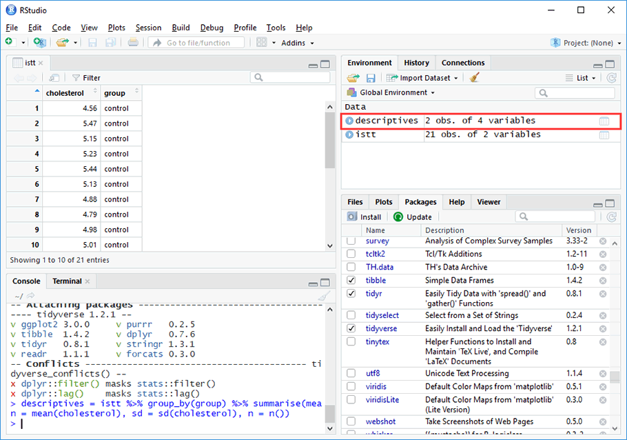
• Press the Enter/Return key on your keyboard to store the data for descriptives in RStudio. You will see a new entry appear in the area under the tab, which describes the data/results that has been stored, including the name of the data (i.e., descriptives), number of rows (i.e., 2 obs., which indicates that there are 2 rows) and number of columns (i.e., 4 variables, which indicates that there are 4 columns) of the table where the data/results are being stored (i.e., the red rectangle highlighted below). In the next step, you will be shown how to display this table of the mean, standard deviation and sample size for each of your two groups.

  

• Enter the following R code into the RStudio Console (i.e., under the tab):

  descriptives

  or

  View(descriptives)

  This R code has the following meaning:

  descriptives

  View the results for descriptives (i.e., descriptives is the label we gave to the object that stored our statistical analysis in Step 3 earlier). Entering descriptives by itself will output the mean, standard deviation and sample size in the RStudio Console (i.e., under the tab).

  View()

  Display the results in the RStudio Source window for the statistical analysis described between the brackets (). Enter this R code exactly as shown without making any changes. Notice that the "V" in View is capitalised (i.e., uppercase). You will get an error if you use a lowercase "v". In other words, when using View() the results will be displayed in the Source window instead of in the RStudio Console. The Source window is highlighted in the next step.

• Press the Enter/Return key on your keyboard to view the mean, standard deviation and sample size for each of your two groups.

  If you entered descriptives in the previous step, the following output is generated by RStudio in the area, which includes: (a) the R code that you have just carried out (i.e., in the red rectangle); and (b) the mean, standard deviation and sample size for each of your two groups (i.e., the blue rectangle):

  

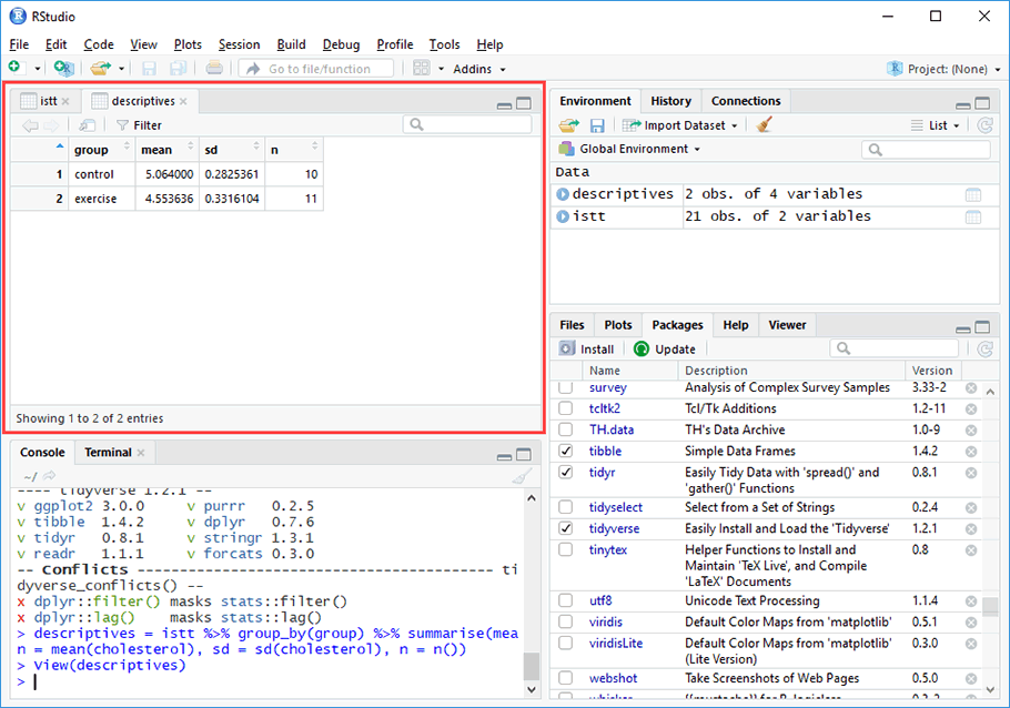
  Alternatively, if you entered View(descriptives) in the previous step, the following table is generated by RStudio in the Source window, which includes the mean, standard deviation and sample size for each of your two groups (i.e., in the red rectangle):

  

• The code to generate the mean difference between your two groups using R, which is simply the difference between the two group mean generated in the previous step, is as follows:

  mean_difference = object[1,2] - object[2,2]

  More specifically, this R code has the following meaning:

  mean_difference =	Give the mean difference you are about to generate a "label" (i.e., a name). For simplicity, we will call it mean_difference. In other words, you are about to calculate the mean difference between the two group means that follow the equals (=) sign. Notice that an equal (=) sign is entered at the end of this R code. Note: If you give your label a different name (e.g., difference_score or md), make sure you do not use a space in the R code (e.g., difference score) because this will produce an error when you try to run your analysis.
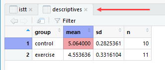
  object[1,2]	Find the statistic (i.e., the mean in this case) along row 1 under column 2 (i.e., denoted by [1,2] in the R code) of the object (i.e., the analysis that was stored) in the previous step. Note that we gave the object the label: descriptives. The statistic is highlighted in red in the Source window below (i.e., if you ran View(descriptives) in the previous step): The statistic is also highlighted in red in the Console window below (i.e., if you ran descriptives in the previous step): Note: In both the Source window and Console window above you can see that the table has two rows (i.e., "1" and "2") and four columns (i.e., "group", "mean", "sd" and "n"). Also, you can see that we have highlighted row 1 and column 2 (i.e., in blue) and the statistic, which is the mean (i.e., in red). In other words, the R code object[1,2] is simply telling RStudio to find the mean score of the dependent variable for the "control" group, which in our example, is 5.06 mmol/L (to 2 decimal places). Therefore, replace object with the label you gave your analysis in the previous step (e.g., descriptives in our example). For [1,2], enter this exactly as shown without making any changes.
  -	Subtract (-) the statistic (i.e., the mean in our case) that follows the minus (-) sign from the statistic in object[1,2]. Enter this R code exactly as shown without making any changes. Note: Make sure that you enter a minus (-) sign and not the longer dash (–) because this is produce an error when you try to run your analysis.
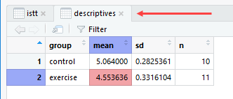
  object[2,2]	Find the statistic (i.e., the mean in this case) along row 2 under column 2 (i.e., denoted by [2,2] in the R code) of the object in the previous step. Remember that we gave the object the label: descriptives. The statistic is highlighted in red in the Source window below (i.e., if you ran View(descriptives) in the previous step): The statistic is also highlighted in red in the Console window below (i.e., if you ran descriptives in the previous step): Note: In both the Source window and Console window above you can see that the table has two rows (i.e., "1" and "2") and four columns (i.e., "group", "mean", "sd" and "n"). Also, you can see that we have highlighted row 2 and column 2 (i.e., in blue) and the statistic, which is the mean (i.e., in red). In other words, the R code object[2,2] is simply telling RStudio to find the mean score of the dependent variable for the "exercise" group, which in our example, is 4.55 mmol/L (to 2 decimal places). Therefore, replace object with the label you gave your analysis in the previous step (e.g., descriptives in our example). For [2,2], enter this exactly as shown without making any changes.

• Using the instructions above, we entered the following R code into the RStudio Console (i.e., under the tab):

  mean_difference = descriptives[1,2] - descriptives[2,2]

  Therefore, the R code above is telling RStudio to calculate the mean difference between the two groups of our independent variable, group (i.e., the "control" and "exercise" groups of our exercise trial) in terms of the scores of our dependent variable, cholesterol (i.e., the cholesterol of participants, measured in mmol/L). The R code is calculating the mean difference by subtracting the mean of the "exercise" group from the mean of the "control" group. Therefore, the mean difference is 0.51 mmol/L (i.e., 5.064000 – 4.553636 = 0.5103636, which is 0.51 to 2 decimal places).

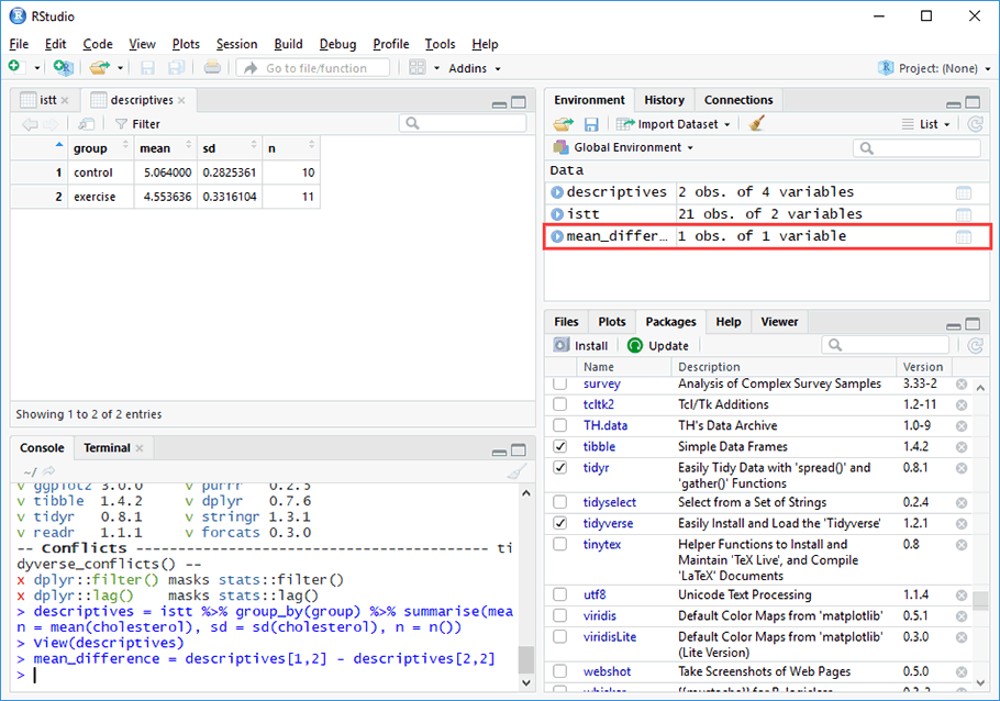
• Press the Enter/Return key on your keyboard to store the data for mean_difference in RStudio. You will see a new entry appear in the area under the tab, which describes the data/result that has been stored, including the name of the data (i.e., mean_difference, which might be shortened, such as mean_differ…), number of rows (i.e., 1 obs., which means 1 row) and number of columns (i.e., 1 variable, which means 1 columns) of the table where the data/result is being stored (i.e., the red rectangle highlighted below). In the next step, you will be shown how to display this table of the mean difference between your two groups.

  

• Enter the following R code into the RStudio Console (i.e., under the tab):

  mean_difference

  or

  View(mean_difference)

  This R code has the following meaning:

  mean_difference

  View the results for mean_difference, which is the mean difference between the two group means. Entering mean_difference by itself will output the mean difference in the RStudio Console (i.e., under the tab).

  View()

  Display the results in the RStudio Source window for the statistical analysis described between the brackets (). Enter this R code exactly as shown without making any changes. Notice that the "V" in View is capitalised (i.e., uppercase). You will get an error if you use a lowercase "v". In other words, when using View() the results will be displayed in the Source window instead of in the RStudio Console. The Source window is highlighted in the next step.

• Press the Enter/Return key on your keyboard to generate the mean difference between your two groups.

  If you entered mean_difference in the previous step, the following output is generated by RStudio in the area, which includes: (a) the R code that you have just run (i.e., in the red rectangle); and (b) the mean difference between your two groups (i.e., in the blue rectangle):

  

  Alternatively, if you entered View(mean_difference) in the previous step, the following table is generated by RStudio in the Source window, which includes the mean difference between your two groups (i.e., in the red rectangle):

  

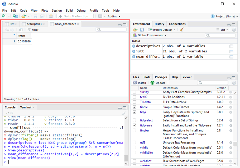
You have now run the independent-samples t-test and generated useful descriptive statistics to help you determine whether there is a statistically significant difference between the two groups of your independent variable in terms of your dependent variable. On the next page we explain how to interpret these results.