Sphericity
Introduction
ANOVAs with repeated measures (within-subject factors) are particularly susceptible to the violation of the assumption of sphericity. Sphericity is the condition where the variances of the differences between all combinations of related groups (levels) are equal. Violation of sphericity is when the variances of the differences between all combinations of related groups are not equal. Sphericity can be likened to homogeneity of variances in a between-subjects ANOVA.
The violation of sphericity is serious for the repeated measures ANOVA, with violation causing the test to become too liberal (i.e., an increase in the Type I error rate). Therefore, determining whether sphericity has been violated is very important. Luckily, if violations of sphericity do occur, corrections have been developed to produce a more valid critical F-value (i.e., reduce the increase in Type I error rate). This is achieved by estimating the degree to which sphericity has been violated and applying a correction factor to the degrees of freedom of the F-distribution. We will discuss this in more detail later in this guide. Firstly, we will illustrate what sphericity is by way of an example.
An Example of Sphericity
To illustrate the concept of sphericity as equality of variance of the differences between each pair of values, we will analyse the fictitious data in the Table 1 below. This data is from a fictitious study that measured aerobic capacity (units: ml/min/kg) at three time points (Time 1, Time 2, Time 3) for six subjects.

Firstly, as we are interested in the differences between related groups (time points), we must calculate the differences between each combination of related group (time point) (the last three columns in the table above). The more time points (or conditions), the greater the number of possible combinations. For three time points, we have three different combinations. We then need to calculate the variance of each group difference, again presented in the table above. Looking at our results, at first glance, it would appear that the variances between the paired differences are not equal (13.9 vs. 17.4 vs. 3.1); the variance of the difference between Time 2 and Time 3 is much less than the other two combinations. This might lead us to conclude that our data violates the assumption of sphericity. We can, however, test our data for sphericity using a formal test called Mauchly's Test of Sphericity.
Testing for Sphericity: Mauchly's Test of Sphericity
As just mentioned, Mauchly's Test of Sphericity is a formal way of testing the assumption of sphericity. Although this test has been heavily criticised, often failing to detect departures from sphericity in small samples and over-detecting them in large samples, it is nonetheless a commonly used test. This is probably due to its automatic print out in SPSS for repeated measures ANOVAs and the lack of an otherwise readily available test. However, despite these shortcomings, because it is widely used, we will explain the test in this section and how to interpret it.
Mauchly's Test of Sphericity tests the null hypothesis that the variances of the differences are equal. Thus, if Mauchly's Test of Sphericity is statistically significant (p < .05), we can reject the null hypothesis and accept the alternative hypothesis that the variances of the differences are not equal (i.e., sphericity has been violated). Results from Mauchly's Test of Sphericity are shown below for our example data (see the red section below):
The results of this test show that sphericity has not been violated (p = .188) (you need to look under the "Sig." column). We can thus report the result of Mauchly's Test of Sphericity as follows:
Mauchly's Test of Sphericity indicated that the assumption of sphericity had not been violated, χ2(2) = 3.343, p = .188.
You might have noticed the discrepancy between the result of Mauchly's Test of Sphericity, which indicates that the assumption of sphericity is not violated, and the large differences in the variances calculated earlier (13.9 vs. 17.4 vs. 3.1), suggesting violation of the assumption of sphericity. Unfortunately, this is one of the problems of Mauchly's test when dealing with small sample sizes, which was mentioned earlier.
If your data does not violate the assumption of sphericity, you do not need to modify your degrees of freedom. [If you are using SPSS, your results will be presented in the "sphericity assumed" row(s).] Not violating this assumption means that the F-statistic that you have calculated is valid and can be used to determine statistical significance. If, however, the assumption of sphericity is violated, the F-statistic is positively biased rendering it invalid and increasing the risk of a Type I error. To overcome this problem, corrections must be applied to the degrees of freedom (df), such that a valid critical F-value can be obtained. It should be noted that it is not uncommon to find that sphericity has been violated.
The corrections that you will encounter to combat the violation of the assumption of sphericity are the lower-bound estimate, Greenhouse-Geisser correction and the Huynh-Feldt correction. These corrections rely on estimating sphericity.
Estimating Sphericity (ε) and How Corrections Work
The degree to which sphericity is present, or not, is represented by a statistic called epsilon (ε). An epsilon of 1 (i.e., ε = 1) indicates that the condition of sphericity is exactly met. The further epsilon decreases below 1 (i.e., ε < 1), the greater the violation of sphericity. Therefore, you can think of epsilon as a statistic that describes the degree to which sphericity has been violated. The lowest value that epsilon (ε) can take is called the lower-bound estimate. Both the Greenhouse-Geisser and the Huynd-Feldt procedures attempt to estimate epsilon (ε), albeit in different ways (it is an estimate because we are dealing with samples, not populations). For this reason, the estimates of sphericity (ε) tend to always be different depending on which procedure is used. By estimating epsilon (ε), all these procedures then use their sphericity estimate (ε) to correct the degrees of freedom for the F-distribution. As you will see later on in this guide, the actual value of the F-statistic does not change as a result of applying the corrections.
So what effect are the corrections on the degrees of freedom having? The answer to this lies in how the critical values for the F-statistic are calculated. The corrections affect the degrees of freedom of the F-distribution, such that larger critical values are used (i.e., the p-value increases). This is to counteract the fact that when the assumption of sphericity is violated, there is an increase in Type I errors due to the critical values in the F-table being too small. These corrections attempt to correct this bias.
Recall that the degrees of freedom used in the calculation of the F-statistic in a repeated measures ANOVA are:
where k = number of repeated measures and n = number of subjects. The three corrections (lower-bound estimate, Greenhouse-Geisser and Huynh-Feldt correction) all alter the degrees of freedom by multiplying these degrees of freedom by their estimated epsilon (ε) as below:
Please note that the different corrections use different mathematical symbols for estimated epsilon (ε), which will be shown later on.
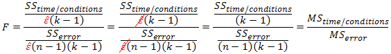
Also recall that the F-statistic is calculated as:
As stated earlier, these corrections do not lead to a different F-statistic. But how does the F-statistic remain unaffected when the degrees of freedom are being altered? This is because the estimated epsilon is added as a multiplier to the degrees of freedom for both the numerator and denominator, and thus they cancel each other out, as shown below:
For our example, we have the three estimates of epsilon (ε) calculated as follows (using SPSS):
Lower-Bound Estimate
The lowest value that epsilon (ε) can take is called the lower-bound estimate (or the lower-bound adjustment) and is calculated as:
where k = number of repeated measures. As you can see from the above equation, the greater the number of repeated measures, the greater the potential for the violation of sphericity. So, for our example which has three repeated measures, the lowest value epsilon (ε) can take would be:
This represents the greatest possible violation of sphericity. Therefore, using the lower-bound estimate means that you are correcting your degrees of freedom for the "worst case scenario". This provides a correction that is far too conservative (incorrectly rejecting the null hypothesis). This correction has been superseded by the Greenhouse-Geisser and Huynd-Feldt corrections, and the lower-bound estimate is no longer a recommended correction (i.e., do not use the lower-bound estimate).
The other types of correction and interpreting statistical printouts of sphericity are to be found on the next page.