Login

Sphericity (cont...)

Greenhouse-Geisser Correction

The Greenhouse-Geisser procedure estimates epsilon (referred to as Greenhouse-Geisser Estimate Epsilon) in order to correct the degrees of freedom of the F-distribution as has been mentioned previously, and shown below:

Corrections to the Degrees of Freedom of the F-distribution

Using our prior example, and if sphericity had been violated, we would have:

Greenhouse-Geisser Estimate to Degrees of Freedom

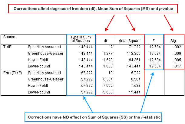
So our F-test result is corrected from F (2,10) = 12.534, p = .002 to F (1.277,6.384) = 12.534, p = .009 (degrees of freedom are slightly different due to rounding). The correction has elicited a more accurate significance value. It has increased the p-value to compensate for the fact that the test is too liberal when sphericity is violated.

Huynd-Feldt Correction

As with the Greenhouse-Geisser correction, the Huynd-Feldt correction estimates epsilon (represented as Huynd-Feldt Estimate Epsilon) in order to correct the degrees of freedom of the F-distribution as shown below:

Huynd-Feldt Estimate to Degrees of Freedom

Using our prior example, and if sphericity had been violated, we would have:

Huynd-Feldt Estimate to Degrees of Freedom

So our F test result is corrected from F (2,10) = 12.534, p = .002 to F (1.520,7.602) = 12.534, p = .005 (degrees of freedom are slightly different due to rounding). As with the Greenhouse-Geisser correction, this correction has elicited a more accurate significance value; it has increased the p-value to compensate for the fact that the test is too liberal when sphericity is violated.

Join the 10,000s of students, academics and professionals who rely on Laerd Statistics.TAKE THE TOUR

Greenhouse-Geisser vs. Huynd-Feldt Correction

The Greenhouse-Geisser correction tends to underestimate epsilon (ε) when epsilon (ε) is close to 1 (i.e., it is a conservative correction), whilst the Huynd-Feldt correction tends to overestimate epsilon (ε) (i.e., it is a more liberal correction). Generally, the recommendation is to use the Greenhouse-Geisser correction, especially if estimated epsilon (ε) is less than 0.75. However, some statisticians recommend using the Huynd-Feldt correction if estimated epsilon (ε) is greater than 0.75. In practice, both corrections produce very similar corrections, so if estimated epsilon (ε) is greater than 0.75, you can equally justify using either.

Interpreting Statistical Printouts

To see all the above in action, consider the data set we have been using for this article. We can see from our earlier table that, for our data set, the estimated epsilon (ε) using the Greenhouse-Geisser method is 0.638 (i.e., Greenhouse-Geisser Estimate Epsilon = 0.638). The following table shows the output of our repeated measures ANOVA (in SPSS):

SPSS Output Repeated Measures ANOVA - Sphericity

In SPSS, the "Sphericity Assumed" row(s) are where sphericity has not been violated, and therefore, represents the normal calculations we would make to calculate a significance value for a repeated measures ANOVA. Notice how the sum of squares and F-statistic are identical regardless of whether or which correction is applied (shown below in blue). This further highlights that the corrections are not being applied to the partitioning of sum of squares, but to the degrees of freedom.

Testimonials
TAKE THE TOUR


Marked Up - SPSS Output Repeated Measures ANOVA - Sphericity

We can see in the diagram above that the corrections have altered the degrees of freedom (df), which in turn have altered the Mean Sum of Squares (MS) for both the TIME factor and its error, and have altered the level of significance of the F-statistic.

Univariate vs. Multivariate Analysis

An alternative method is to use a MANOVA instead of a repeated measures ANOVA. The reason for doing this is that the MANOVA does not require the assumption of sphericity. There are a number of reasons for choosing a MANOVA over a repeated measures ANOVA and vice versa, and we will be adding this information to this guide soon.

« prev
1 2