Spearman's Correlation using Stata

Introduction

The Spearman rank-order correlation coefficient (shortened to Spearman’s rank correlation in Stata) is a nonparametric test which measures the strength and direction of association between two variables that are measured on an ordinal or continuous scale. The Spearman correlation coefficient is often denoted by the symbol r_s (or the Greek letter ρ, pronounced rho). It is a useful test when Pearson's correlation cannot be run due to violations of normality, a non-linear relationship or when ordinal variables are being used.

For example, you could use a Spearman's correlation to understand whether there is an association between high jump performance and time spent training (i.e., your two variables would be "high jump performance", measured in height jumped, and "time spent training", measured in hours per week). If there was a moderate, positive association, we could say that more time spent training was associated with better high jump performance. Alternately, you could use a Spearman's correlation to understand whether there is an association between length of unemployment and health (i.e., your two variables would be "length of unemployment", measured in days, and "health", measured using a continuous scale). If there was a strong, negative association, we could say that the longer the length of unemployment, the lower the level of health.

In this guide, we show you how to carry out a Spearman's correlation using Stata, as well as interpret and report the results from this test. However, before we introduce you to this procedure, you need to understand the different assumptions that your data must meet in order for a Spearman's correlation to give you a valid result. We discuss these assumptions next.

Stata

Assumptions

There are two assumptions that underpin a Spearman's correlation. If either of these two assumptions are not met, analysing your data using a Spearman's correlation might not lead to a valid result. Since assumption #1 relates to your choice of variables, it cannot be tested for using Stata. However, you should decide whether your study meets this assumption before moving on.

• Assumption #1: Your two variables should be measured on an ordinal or continuous scale (i.e., interval or ratio scale). Examples of ordinal variables include Likert scales (e.g., a 7-point scale from "strongly agree" through to "strongly disagree"), amongst other ways of ranking categories (e.g., a 5-point scale for measuring job satisfaction, ranging from "most satisfied" to "least satisfied"; a 4-point scale determining how easy it was to navigate a new website, ranging from "very easy" to "very difficult"; or a 3-point scale explaining how much a customer liked a product, ranging from "Not very much" to "Yes, a lot"). Examples of continuous variables include height (measured in feet and inches), temperature (measured in °C), salary (measured in US dollars), revision time (measured in hours), intelligence (measured using IQ score), reaction time (measured in milliseconds), test performance (measured from 0 to 100), sales (measured in number of transactions per month), and so forth. You can learn more about ordinal and continuous variables in our article: Types of Variable.

Fortunately, you can check assumption #2 using Stata. When moving on to assumption #2, do not be surprised if your data fails this assumption since this can happen when working with real-world data rather than textbook examples, which often only show you how to carry out a Spearman's correlation when everything goes well. However, don't worry because even when your data fails this assumption, there is often a solution to overcome this (e.g., transforming your data or using another statistical test instead). Just remember that if you do not check that you data meets this assumption or you do not test for it correctly, the results you get when running a Spearman's correlation might not be valid.

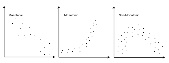
• Assumption #2: There needs to be a monotonic relationship between the two variables. A monotonic relationship exists when either the variables increase in value together, or as one variable value increases, the other variable value decreases. Whilst there are a number of ways to check whether a monotonic relationship exists between your two variables, we suggest creating a scatterplot using Stata where you can plot one variable against the other, and then visually inspect the scatterplot to check for monotonicity. Your scatterplot may look something like one of the following:
  
  

  Copyright © Laerd Statistics 2014

  
  If the relationship displayed in your scatterplot is not monotonic, you will have to consider either a transformation or another type of test entirely. In practice, checking for assumption #2 it is not a difficult task and Stata provides all the tools you need to do this.

It is also worth noting that your variables do not need to be normally distributed to run a Spearman’s correlation. In addition, Spearman's correlation is not very sensitive to outliers (unusual observations in your data), so the presence of these data points does not automatically invalidate the results you get from running a Spearman's correlation.

In the section, Test Procedure in Stata, we illustrate the Stata procedure required to perform a Spearman's correlation assuming that no assumptions have been violated. First, we set out the example we use to explain the Spearman's correlation procedure in Stata.

Stata

Example

The value of receiving an education is always in the news, particularly with respect to the salary improvement that can be attained with a "graduate job". As a very simply study, a researcher wanted to know whether the number of years that a person was educated was associated with their salary at 35 years old. To carry out this analysis, the researcher recruited a small sample of 13 participants aged 35 years old. They recorded the number of years of education they had received (entered into the variable, edu_years) and their current salary (entered into the variable, salary). Expressed in variable terms, the researcher wanted to correlate salary and edu_years.

Note: The example and data used for this guide are fictitious. We have just created them for the purposes of this guide. In addition, it was assumed that the data failed the assumptions required for running a Pearson's correlation.

Stata

Setup in Stata

In Stata, we created two variables: (1) salary, which is a participant's salary (in $1,000s per year); and (2) edu_years, which is the number of years of education that a participant has received.

Note: It does not matter which variable you create first.

After creating these two variables – edu_years and salary – we entered their scores into the two columns of the Data Editor (Edit) spreadsheet, as shown below:

Published with written permission from StataCorp LP.

Stata

Test Procedure in Stata

In this section, we show you how to analyse your data using a Spearman's correlation in Stata when the two assumptions described in the previous section, Assumptions, have not been violated. You can carry out a Spearman's correlation using code or Stata's graphical user interface (GUI). After you have carried out your analysis, we show you how to interpret your results. First, choose whether you want to use code or Stata's graphical user interface (GUI).

Code

The basic code to run a Spearman's correlation takes the form:

spearman VariableA VariableB

Using this code, Stata will report: (a) the number of observations (i.e., participants) in the Spearman's correlation analysis; (b) Spearman's correlation coefficient; and (c) its statistical significance (i.e., p-value). There are various other options available in Stata, but we will concentrate on the basic statistics in this guide.

Substituting the two variables in our example – salary and edu_years – into respectively VariableA and VariableB in the code shown above, you get the following code:

spearman salary edu_years

This is the code you need to enter into Stata to run a Spearman's correlation on these variables. Code needs to be entered into the box in Stata, which is shown below:

Published with written permission from StataCorp LP.

Therefore, enter the code into the box, as shown below:

Published with written permission from StataCorp LP.

Now press the "Return/Enter" key on your keyboard to generate the results. The Stata output that will be produced is shown here.

Graphical User Interface (GUI)

The three steps required to carry out a Spearman's correlation in Stata 12 and 13 are shown below:

1. For Stata 13, Click Statistics > Nonparametric analysis > Tests of hypotheses > Spearman's rank correlation on the main menu, as shown below:

   Note: For Stata 12 (but also valid for Stata 13), click Statistics > Summaries, tables, and tests > Nonparametric tests of hypotheses > Spearman's rank correlation on the main menu.

   

   Published with written permission from StataCorp LP.

   
   You will be presented with the following spearman - Spearman's rank correlation coefficients dialogue box:
   
   

   Published with written permission from StataCorp LP.

2. Select salary and edu_years from within the Variables: (leave empty for all) box, using the button. You will end up with the following screen:
   

   Published with written permission from StataCorp LP.

   Note: It does not matter in which order you select your two variables from within the Variables: (leave empty for all) box. In addition, if you select all the options in the –List of Statistics– area, you will end up with the same output (i.e., the sample size, Spearman's correlation coefficient and statistical significance level.

3. Click on the button. This will generate the output.

Stata

Output of a Spearman's correlation in Stata

If your data passed assumption #2 (i.e., there was a monotonic relationship between your two variables), which we explained earlier in the Assumptions section, you will only need to interpret the following Spearman's correlation output in Stata:

Published with written permission from StataCorp LP.

The first line (i.e., "spearman edu_years salary") contains the code that Stata ran to generate a Spearman's correlation. If you followed the code approach (here) you will recognize this as the code you entered into Stata. On the other hand, GUI users will not recognize this code, but this is the code that was run behind the scenes when you selected the various options in the spearman - Spearman's rank correlation coefficients dialogue box.

The next line ("Number of obs = 13") contains the number of observations (i.e., participants) that were analysed. There were 13 participants in this example; hence "13" in the output. The next line ("Spearman's rho = 0.8583") presents the actual value for Spearman's correlation coefficient. You can see that Spearman's rho (ρ) is 0.8583. Values for Spearman's correlation coefficient are generally less than for Pearson's correlation coefficient and a Spearman's ρ of 0.8583 indicates a strong monotonic relationship. As Spearman's coefficient is positive you can conclude that a greater number of years in education is associated with a larger salary. The last line ("Prob > |t| = 0.0002") of the output presents the two-tailed statistical significance (i.e., p-value) of the Spearman's correlation coefficient. You can see that Spearman's correlation coefficient is statistically significant because p = .0002, which is less than p < .05 (a common threshold for statistical significance).

Stata

Reporting a Spearman's correlation

When you report the output of your Spearman's correlation, it is good practice to include:

• A. An introduction to the analysis you carried out.
• B. Information about your sample (including any missing values).
• C. The Spearman correlation coefficient, r_s.
• C. The statistical significance level (i.e., p-value) of your result.

Based on the results above, we could report the results of this study as follows:

In addition to the reporting the results as above, a diagram can be used to visually present your results. For example, you could do this using a scatterplot. This can make it easier for others to understand your results and is easily produced in Stata.