Two-way ANOVA in SPSS Statistics (cont...)
Interpreting the SPSS Statistics output of the two-way ANOVA
SPSS Statistics generates quite a few tables in its output from a two-way ANOVA. In this section, we show you the main tables required to understand your results from the two-way ANOVA, including descriptives, between-subjects effects, Tukey post hoc tests (multiple comparisons), a plot of the results, and how to write up these results.
For a complete explanation of the output you have to interpret when checking your data for the six assumptions required to carry out a two-way ANOVA, see our enhanced guide. This includes relevant boxplots, and output from your Shapiro-Wilk test for normality and test for homogeneity of variances.
Finally, if you have a statistically significant interaction, you will also need to report simple main effects. Alternatively, if you do not have a statistically significant interaction, there are other procedures you will have to follow. We show you these procedures in SPSS Statistics, as well as how to interpret and write up your results in our enhanced two-way ANOVA guide.
Below, we take you through each of the main tables required to understand your results from the two-way ANOVA.
SPSS Statistics
Descriptive statistics
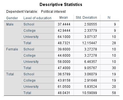
You can find appropriate descriptive statistics for when you report the results of your two-way ANOVA in the aptly named "Descriptive Statistics" table, as shown below:

Published with written permission from SPSS Statistics, IBM Corporation.
This table is very useful because it provides the mean and standard deviation for each combination of the groups of the independent variables (what is sometimes referred to as each "cell" of the design). In addition, the table provides "Total" rows, which allows means and standard deviations for groups only split by one independent variable, or none at all, to be known. This might be more useful if you do not have a statistically significant interaction.
SPSS Statistics
Plot of the results
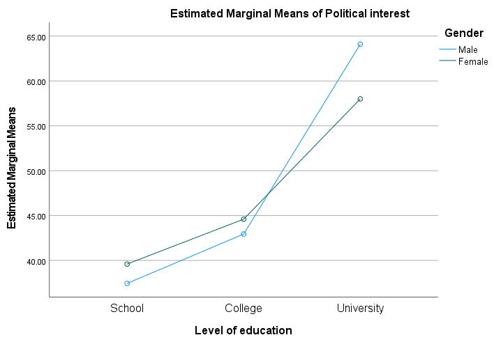
The plot of the mean "interest in politics" score for each combination of groups of "gender" and "education_level" are plotted in a line graph, as shown below:
Published with written permission from SPSS Statistics, IBM Corporation.
Although this graph is probably not of sufficient quality to present in your reports (you can edit its appearance in SPSS Statistics), it does tend to provide a good graphical illustration of your results. An interaction effect can usually be seen as a set of non-parallel lines. You can see from this graph that the lines do not appear to be parallel (with the lines actually crossing). You might expect there to be a statistically significant interaction, which we can confirm in the next section.
SPSS Statistics
Statistical significance of the two-way ANOVA
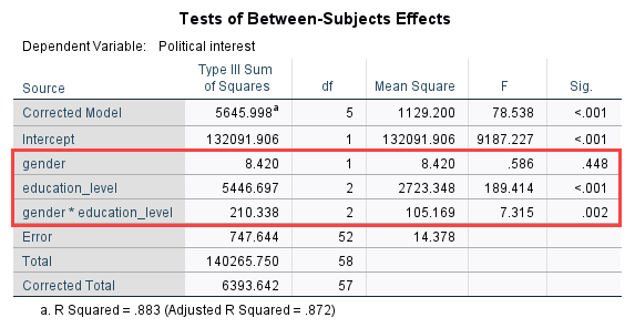
The actual result of the two-way ANOVA – namely, whether either of the two independent variables or their interaction are statistically significant – is shown in the Tests of Between-Subjects Effects table, as shown below:
Published with written permission from SPSS Statistics, IBM Corporation.
The particular rows we are interested in are the "gender", "education_level" and "gender*education_level" rows, and these are highlighted above. These rows inform us whether our independent variables (the "gender" and "education_level" rows) and their interaction (the "gender*education_level" row) have a statistically significant effect on the dependent variable, "interest in politics". It is important to first look at the "gender*education_level" interaction as this will determine how you can interpret your results (see our enhanced guide for more information). You can see from the "Sig." column that we have a statistically significant interaction at the p = .002 level. You may also wish to report the results of "gender" and "education_level", but again, these need to be interpreted in the context of the interaction result. We can see from the table above that there was no statistically significant difference in mean interest in politics between males and females (p = .448), but there were statistically significant differences between educational levels (p < .001).
SPSS Statistics
Post hoc tests – simple main effects in SPSS Statistics
When you have a statistically significant interaction, reporting the main effects can be misleading. Therefore, you will need to report the simple main effects. In our example, this would involve determining the mean difference in interest in politics between genders at each educational level, as well as between educational level for each gender. If you have SPSS Statistics versions 28 to 30 (or the subscription version of SPSS Statistics), you can carry out a simple main effects analysis using the graphical user interface (i.e., the dialogue boxes in SPSS Statistics). However, if you have SPSS Statistics version 27 or an earlier version of SPSS Statistics, you can still carry out a simple main effects analysis, but you will need to use SPSS Statistics syntax. Therefore, in our enhanced two-way ANOVA guide, we show you the procedure for doing this in SPSS Statistics, as well as explaining how to interpret and write up the output from your simple main effects.
When you do not have a statistically significant interaction, we explain two options you have, as well as a procedure you can use in SPSS Statistics to deal with this issue.
SPSS Statistics
Multiple Comparisons Table
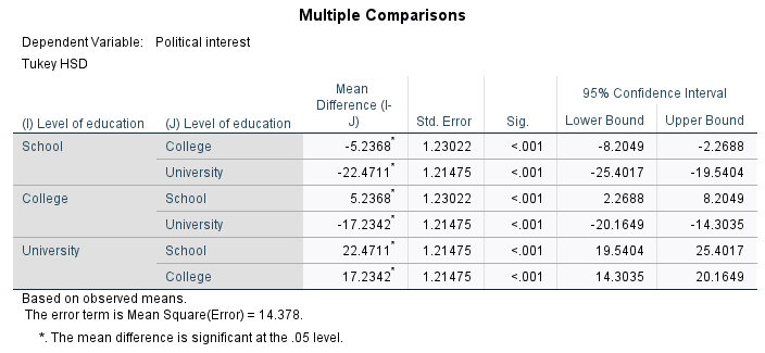
If you do not have a statistically significant interaction, you might interpret the Tukey post hoc test results for the different levels of education, which can be found in the Multiple Comparisons table, as shown below:
Published with written permission from SPSS Statistics, IBM Corporation.
You can see from the table above that there is some repetition of the results, but regardless of which row we choose to read from, we are interested in the differences between (1) School and College, (2) School and University, and (3) College and University. From the results, we can see that there is a statistically significant difference between all three different educational levels (p < .001).
SPSS Statistics
Reporting the results of a two-way ANOVA analysis
You should emphasize the results from the interaction first before you mention the main effects. For example, you might report the result as:
A two-way ANOVA was conducted that examined the effect of gender and education level on interest in politics. There was a statistically significant interaction between the effects of gender and education level on interest in politics, F (2, 52) = 7.315, p = .002.
If you had a statistically significant interaction term and carried out the procedure for simple main effects in SPSS Statistics, you would also report these results. Briefly, you might report these as:
Simple main effects analysis showed that males were significantly more interested in politics than females when educated to university level (p = .002), but there were no differences between gender when educated to school (p = .465) or college level (p = .793).
In our enhanced two-way ANOVA guide, we show you how to write up the results from your assumptions tests and two-way ANOVA procedure, including simple main effects, if you need to report this in a dissertation/thesis, assignment or research report. We do this using the Harvard and APA styles. You can learn more about our enhanced content on our Features: Overview page.