Repeated measures logistic regression using generalized estimating equations (GEE)
Introduction
A repeated measures logistic regression is used to understand if there are differences between two or more independent groups (e.g., a "control group" and an "intervention group", "males" and "females") across two or more repeated measurements (e.g., multiple "time points" over a year, "multiple conditions/treatments" that subjects undergo) when the dependent variable is dichotomous (e.g., a fitness test is "passed" or "failed", cholesterol concentration is "above" or "below" a specific value after taking the new drug).
Note: If you have a similar study design, but your dependent variable is continuous rather than dichotomous, see our SPSS Statistics guide on the mixed ANOVA.
In the tabs below, we set out two examples where a repeated measures logistic regression could be used: (a) where the repeated measurements are multiple time points (e.g., "before" and "after" an exercise intervention, "every month" for a year after taking a new drug); and (b) where the repeated measurements are multiple conditions/treatments (e.g., subjects take "four doses" of a migraine drug to measure adverse drug reactions, "three types" of energy drink are imbibed by subjects to measure driving alertness):
- The repeated measurements are multiple time points
- The repeated measurements are multiple conditions/treatments
The repeated measurements are multiple time points
Your within-subjects factor is time.
Your between-subjects factor consists of conditions (also known as treatments).
Imagine that a researcher working for a consumer watchdog wants to help learner drivers understand how many hours of driving lessons they should purchase in order to pass their driving test. The researcher also wants to understand if there is a difference based on whether the learner has manual driving lessons (known as "stick shift" in the United States) or automatic driving lessons.
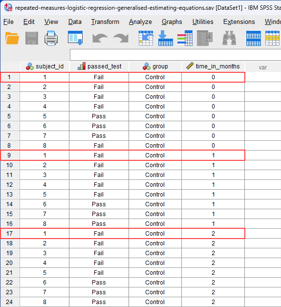
To achieve this, the researcher sets up an experiment where 100 learner drivers are randomly assigned to one of two treatment/experimental groups: "manual/stick shift driving lessons" and "automatic driving lessons". All 100 learners are given 40 hours of driving lessons. At the end of every 5 hours of driving, the instructor gives each learner a 30-minute "mock driving test", which they can either "pass" or "fail". Therefore, the learners take a total of 8 mock driving tests (i.e., 40 hours of lessons divided by 5 hours = 8 mock tests).
The researcher wanted learners to be tested after every extra 5 hours of driving because driving lessons are typically booked in "blocks" (e.g., blocks of 5, 10 or 20 hours of lessons). Therefore, the researcher wanted to use the smallest block (i.e., 5 hour blocks) because the goal of the research was to save learners money (i.e., learners are encouraged to buy bigger blocks of driving lessons with discounted prices, but this could still cost more overall if learner drivers do not need so many lessons).
In this example, the dichotomous dependent variable is "driving test", which has two groups: "pass" and "fail". The within-subjects factor (also known as a repeated measures independent variable) is "time", with "8 time points" (i.e., where learners are given a mock driving tests at the end of each 5 hours of driving lessons). The between-subjects factor is "lesson type", which has two independent groups: "manual/stick shift" and "automatic" (i.e., the two groups are "independent" because a learner can only be in one of these two groups).
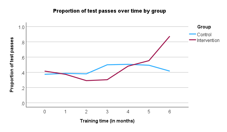
At the end of the experiment, the researcher starts by describing the proportion of "passes" and "fails" over the 8 mock driving tests between manual/stick shift and automatic learners. For example, in the 1st mock driving test, the "pass" rate was .0 (i.e., 0%) for manual/stick shift learners and .0 (i.e., 0%) for automatic learners. In other words, none of the learners passed the mock test after their first 5 hours of driving lessons, which is perhaps not surprising. By comparison, by the 8th mock driving test, the "pass" rate was .634 (i.e., 63.4%) for manual/stick shift learners and .701 (i.e., 70.1%) for automatic learners. Expressed another way, the "fail" rate was .366 (i.e., 36.6%) for manual/stick shift learners and .299 (i.e., 29.9%) for automatic learners. The researcher presents these "pass" and "fail" rates for all 8 mock driving tests in a table, which provide useful descriptive statistics to get a sense of the data.
Next, the researcher uses a repeated measures logistic regression using generalized estimating equations (GEE) to determine whether there is a difference in the proportion of "passes" over the 8 mock driving tests between manual/stick shift and automatic learners. In other words, is there a two-way interaction effect between "time" and "lesson type" in terms of the dependent variable, which is the proportion of learners who "pass" each mock driving test? If there is a two-way interaction effect, this suggests that the proportion of passes and fails is not the same over time for manual/stick shift and automatic learners. In other words, how learners improve after each 5 hours of extra driving lessons, assessed in terms of the proportion of "passes", is not the same for manual/stick shift learners compared to learners who had automatic lessons. The researcher can also use follow-up analyses to understand how pass rates might change over time for manual/stick shift and automatic learners. For example, the researcher may want to understand how pass rates changed for manual/stick shift and automatic learners for every extra 5 hours driving lessons.
The repeated measurements are multiple conditions/treatments
Your within-subjects factor consists of conditions (also known as treatments).
Your between-subjects factor is a characteristic of your sample.
A national health service wants to review the adverse side effects of three migraine drugs that its doctors prescribe to patients with long-term (chronic) migraine. The health service wants to determine the proportion of patients who experience an "adverse drug reaction (ADR)" after taking the drugs. Whilst there are different types of adverse drug reaction (ADR), for the purpose of this example, we are referring to "Type A" reactions (e.g., see MHRA, 2025). The health service is also interested in differences in ADR between males and females.
To achieve this, a researcher from the health service sets up a study where 120 migraine patients are prescribed each of the three drugs for a 3-month period. For the simplicity of this example, the order that the patients receive the three drugs is random to try to avoid "order effects" and there is a "washout period" between each trial to ensure that the effects of each drug are no longer present before the next drug is prescribed. If a patient experiences an ADR whilst taking a drug, the trial is stopped and the patients starts the washout period before starting the next drug.
In this example, the dichotomous dependent variable is "ADR", which has two groups: "no" and "yes". The within-subjects factor (also known as a repeated measures independent variable) is "condition/treatment", with "3 repeated measures" (i.e., where patients take 3 different migraine drugs, each for a 3-month period). The between-subjects factor is "gender", which has two independent groups: "males" and "females".
At the end of the experiment, the researcher starts by describing the proportion of male and female patients who experienced an ADR for each of the three migraine drugs. For example, when taking the first migraine drug, .012 (i.e., 1.2%) of males and .024 (i.e., 2.4%) of females experienced an ADR. The researcher presents the proportion of male and female patients who experience an ADR for each of the three migraine drugs in a table, which provide useful descriptive statistics to get a sense of the data.
Next, the researcher uses a repeated measures logistic regression using generalized estimating equations (GEE) to determine whether there is a difference in the proportion of male and female patients who experience an ADR when taking each of the three migraine drugs. In other words, is there a two-way interaction effect between "gender" and "drug" in terms of the dependent variable, which is the proportion of patients who experience an ADR (i.e., who state "yes" to experiencing an ADR)? If there is a two-way interaction effect, this suggests that the proportion of male and female patients who experience an ADR is not the same when taking each of the three migraine drugs. In other words, whether patients experience an ADR after taking each drug differs based on whether they are male or female and the drug that was taken. The researcher can also use follow-up analyses to understand in more detail how the proportion of patients who experience an ADR might differ based on their gender and which of the three migraine drugs they take.
Note: In the examples above, there is one between-subjects factor and one within-subjects factor, which is called a two-way mixed design. However, a repeated measures logistic regression can be used when you have one or more between-subjects factors and one or more within-subjects factors (e.g., a three-way mixed design that can have two between-subjects factors and one within-subjects factor). In this guide, we illustrate the two-way mixed design as an introduction to the use of a repeated measures logistic regression.
There are many methods that can be used when analysing data for a mixed design when the dependent variable is dichotomous. In this guide, we show how to carry out a repeated measures logistic regression using generalized estimating equations (GEE), which we will simply refer to as GEE for the remainder of this guide. However, we also plan to add guides to show how to carry out a repeated measures logistic regression using different methods such as generalized linear mixed models (GLMM). If you would like us to email you when these guides become available, please contact us.
Note: Both the GEE and GLMM methods can be used for a wide range of mixed designs and types of dependent variable (e.g., count, ordinal, nominal, dichotomous and continuous dependent variables). However, in this introductory guide, we illustrate the use of GEE for a two-way mixed design when the dependent variable is dichotomous (i.e., an ordinal or nominal variable with two groups/categories).
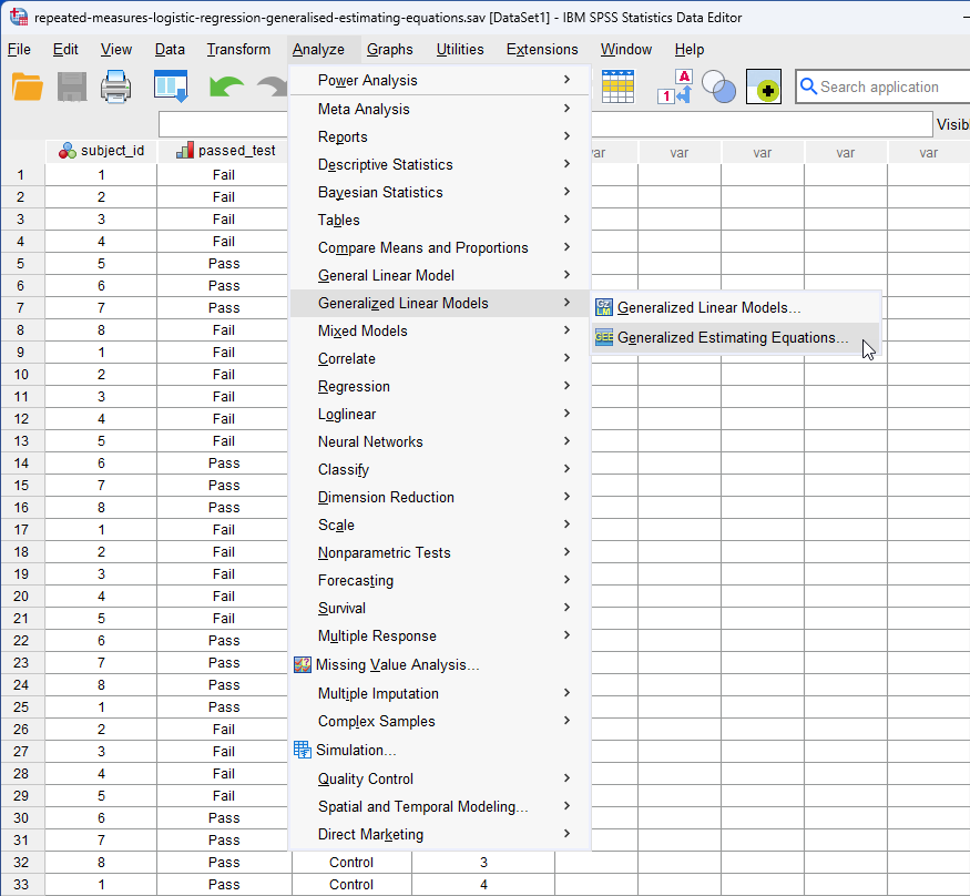
In the sections that follow, we start by setting out the basic requirements and assumptions that underpin a repeated measures logistic regression using GEE when you have a two-way mixed design. It is important that your study design, variables and data fit with these basic requirements and assumptions to ensure that a repeated measures logistic regression using GEE will give you accurate/valid results. Next, we set out the example that is used throughout this guide to illustrate the use of a repeated measures logistic regression using GEE for a two-way mixed design. Third, we show you how to set up your data in SPSS Statistics to carry out this type of analysis. Next, we set out the SPSS Statistics procedure to carry out a repeated measures logistic regression using GEE for a two-way mixed design, which uses the Generalized Estimating Equations procedure in SPSS Statistics. Finally, we explain how to interpret the SPSS Statistics output/results that are produced when running the Generalized Estimating Equations procedure.
Note: We do not currently have a premium version of this guide in the subscription part of our website. However, we plan to add a whole series of detailed guides to help with GEE and GLMM for repeated measures and mixed designs with count, ordinal, nominal, dichotomous and continuous dependent variables. If you would like us to email you when these guides become available, please contact us.
SPSS Statistics
Basic requirements and assumptions of a repeated measures logistic regression using generalized estimating equations (GEE)
When you choose to analyse your data using repeated measures logistic regression using GEE, part of the process involves checking to make sure that the data you want to analyse can actually be analysed using this type of statistical analysis. You need to do this because it is only appropriate to use repeated measures logistic regression using GEE if your data: (a) "meets" three basic requirements that are needed for a repeated measures logistic regression using GEE to be appropriate for your study design and how you measured your variables; and (b) "passes" three assumptions that are required to give you a valid result. These basic requirements and assumptions are set out below:
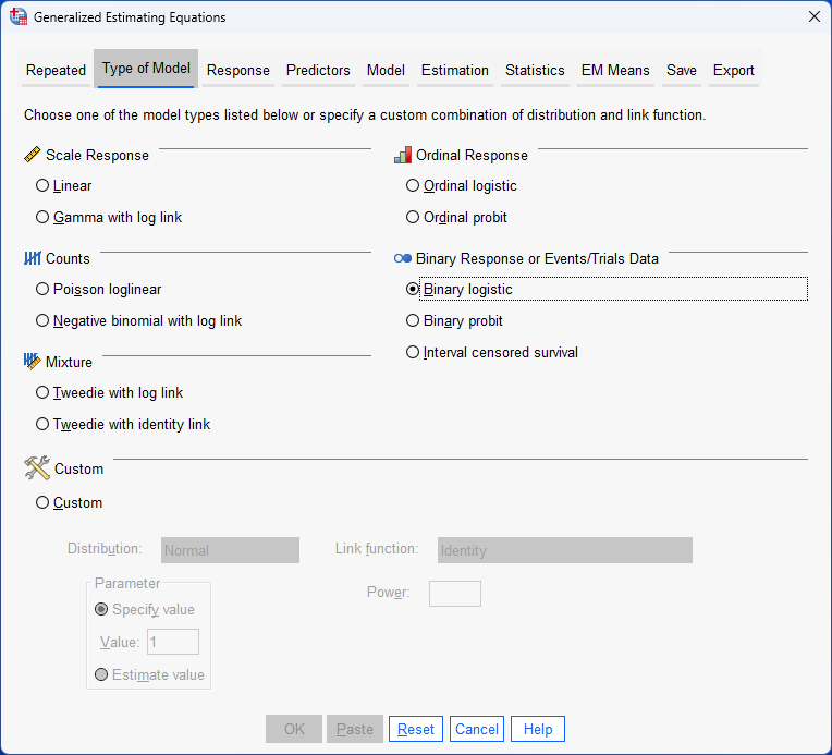
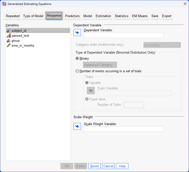
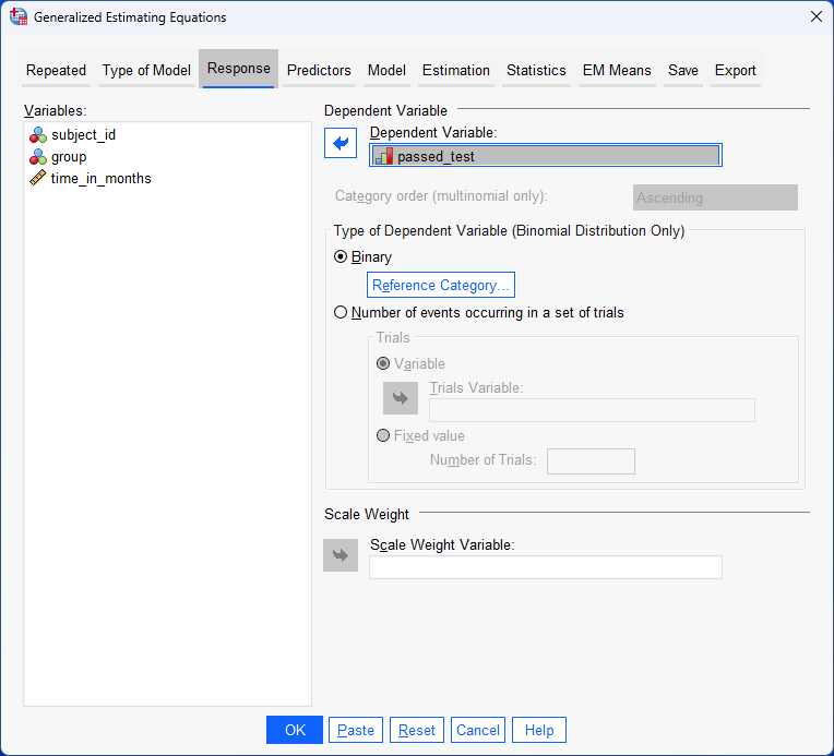
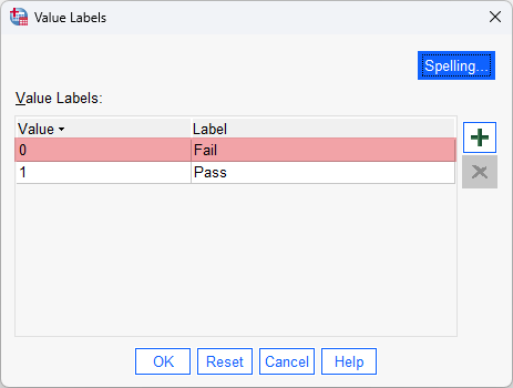
- Requirement #1: Your dependent variable should be measured on a dichotomous scale (i.e., it is a nominal or ordinal variable with two groups/categories).
Examples of dichotomous variables include exam result (two groups: "pass" and "fail"), presence of heart disease (two groups: "yes" and "no"), personality type (two groups: "introversion" and "extroversion"), body composition (two groups: "obese" and "not obese"), brand preference ("Apple" and "Samsung"), and so forth.Note: If your dependent variable is a continuous variable rather than a dichotomous variable, see our guide on the mixed ANOVA. Alternatively, if your dependent variable is a count, or an ordinal or nominal variable with three or more groups/categories, we will be adding SPSS Statistics guides using GEE and GLMM to help with these types of analysis. If you would like us to email you when these guides become available, please contact us.
- Requirement #2: Your within-subjects factor (i.e., repeated measures independent variable) should consist of at least two categorical, related groups.
A within-subjects factor is an independent variable with related groups, where the term "related groups" usually indicates that the same subjects are present in each group. The reason that it is possible to have the same subjects in all groups is because each subject has been measured on two or more occasions using the same dependent variable. These two or more occasions could be: (a) two or more time points where each subject is measured; or (b) two or more conditions/treatments where each subject is measured.
For example, you might have measured 150 students' performance in a spelling test (the dependent variable) before and after they underwent a new form of computerized teaching method to improve spelling (i.e., two different time points). You would like to know if the computer training improved their spelling performance, where the dependent variable has two groups (i.e., the test was "passed" or "failed"). The first related group consists of the subjects at the beginning of the experiment, prior to the computerized spelling training, and the second related group consists of the same subjects, but now at the end of the computerized training. In your study design, you may have only two time points (e.g., before and after an intervention, such as in the new computerized teaching method mentioned above) or a few time points (e.g., every month for a year after taking a new drug). - Requirement #3: Your between-subjects factor (i.e., between-subjects independent variable) should consist of at least two categorical, "independent groups".
A between-subjects factor is an independent variable with independent groups, where the term "independent groups" indicates that different subjects are present in each group.
Examples of between-subjects factors include gender (two groups: "males" and "females"), ethnicity (three groups: "Caucasian", "African American" and "Hispanic"), physical activity level (four groups: "sedentary", "low", "moderate" and "high"), profession (five groups: "surgeon", "doctor", "nurse", "dentist", "therapist"), and so forth. Since the groups are independent and mutually exclusive, a subject cannot be in more than one group. For example, a person cannot be "male" and "female". Alternatively, at the time of starting an exercise experiment, the subject cannot be in the "sedentary" and "high" physical activity groups; they can only be in one of the four physical activity groups: "sedentary", "low", "moderate" or "high".
If your study design and variables does not met any of the three requirements above, a repeated measures logistic regression using GEE would not be a suitable type of analysis. If you are unsure what alternatives are available, please contact us, letting us know which of these requirements were not met. Alternatively, if your study and variables fit with these three requirements, you can continue onto the two assumptions of a repeated measures logistic regression using GEE below:
- Assumption #1: The working correlation matrix is a good fit.
When you have a within-subjects factor, there are repeated measurements, whether these are multiple time points or multiple conditions/treatments. Using the examples discussed earlier, whether learners driver passed or failed a mock driving test was measured 8 times. In the drug example, whether a patient experienced an adverse drug reaction (ADR) was measured when they took 3 different migraine drugs.
Simply stated, when the data is repeatedly sampled from the same participants, there is a lack of independence between the data points (values) for each participant. Instead, there is a dependence/correlation between data points (values) for each participant, such that: (a) each participant is likely to be more similar to themselves than others; and (b) data points closer in time tend to be more similar than data points distant in time. This dependence/correlation needs to be taken into account (Liang & Zeger, 1986; Diggle et al., 2002; Agresti, 2013).
For example, all other things being equal, we would expect to learn more about how much progress a learner driver makes after each extra 5 hours of lessons (i.e., whether they fail or pass the mock test) based on that learners previous success (i.e., whether they failed or passed the mock test in the past) than by comparing them to another learner who has taken the same number of lessons. Also, we would expect the relative success of a learner driver to be more similar when comparing whether they failed or passed the mock test within the previous 5 hours or next 5 hours of driving lessons compared to whether they passed or failed the mock test 20 hours ago or after another 20 hours of driving lessons. As another example, we would expect that knowledge of whether a patient experiences an ADR after taking a drug is more likely to be related to the potential pharmacological effects of that drug on that patient (i.e., how that patient's body responds to the drug) compared to what we would learn from how another patient responds to the same drug (all other things being equal).
To try and take into account the dependence/correlation between data points (values) for a given participant, GEE uses what is called a working correlation matrix. Whilst the underlying correlation structure is unknown (Diggle et al., 2002), there are methods to help you choose a suitable working correlation matrix (Hin & Wang, 2008; Breitung et al., 2010; Ziegler & Vens, 2010; Hardin & Hilbe, 2013; Wang & Fu, 2017; Fu et al., 2018).
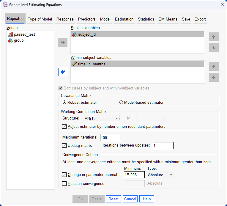
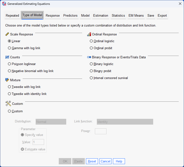
There are many different correlation matrix structures that can be used to best model the data. SPSS Statistics offers five working correlation matrix structures: Independent, AR(1), Exchangeable, M-dependent and Unstructured (IBM Corporation, 2021). Each of these five structures makes different assumptions about the structure of the dependences/correlation between the data points (values) for each participant. As an illustration, we use the AR(1) structure when demonstrating the procedure to carry out a repeated measures logistic regression analysis using GEE later in this guide.Note: If you would like us to add a detailed guide explaining: (a) the different methods to choose a suitable working correlation matrix; and (b) what each of these five correlation matrix structures assume about the data and when they might be the appropriate choice, please contact us.
- Assumption #2: The model fits the data well.
A GEE approach to a repeated measures logistic regression is sensitive to influential points that can distort the overall conclusions from the analysis. For example, extreme outliers might be capable of doing this. To test for model fit, you can use both graphical and numerical methods (e.g., see Hardin & Hilbe, 2013).Note: Again, if you would like us to add a detailed guide explaining the different graphical and numerical methods to test how well the model fits the data, please contact us.
- Assumption #3: Any missing data must be missing completely at random (MCAR).
Missing data can be: (a) intermittent, where a subject misses some time points or conditions/treatments, but not others; or (b) resulting from dropouts, where a subject misses a particular time point or condition/treatment and does not return for future time points or conditions/treatments.
Furthermore, missing data can be classified as missing completely at random (MCAR), missing at random (MAR) and missing not at random (MNAR) (Rubin, 1976). The GEE approach to repeated measures logistic regression can deal with data that is missing completely at random (MCAR). However, the results can be biased if the data is missing at random (MAR). Data that is missing not at random (MNAR) is particularly problematic.
In this guide, we show how to use GEE for a repeated measures logistic regression when the data is at least MCAR (i.e., there is either no missing data or the missing data is MCAR). However, there are methods to deal with MAR data and still use the GEE approach (e.g., Robins and Rotnitzky, 1995; Little and Rubin, 2002, 2020; Preisser et al., 2002).Note 1: If you do not know the difference between data that is MCAR, MAR and MNAR, and would like us to add a guide explaining these types of missing data, please contact us. Similarly, we plan to add guides to help using GEE for a repeated measures logistic regression when the data is MAR. If this is of interest, please contact us and we will let you know when these guides become available.
Note 2: Missing data is not strictly an "assumption" of a GEE analysis. However, we include it because of the negative effect that missing data that is MAR and MNAR will have on the accuracy of your results if not taken into account in your analysis.
You can partially check assumptions #1, #2 and #3 using SPSS Statistics. As for requirements #1, #2 and #3, these should be checked before assumptions #1, #2 and #3 because a repeated measures logistic regression will not be a suitable type of analysis if your study design and variables do not meet these requirements.
In the section, Procedure, we illustrate the SPSS Statistics procedure to perform a repeated measures logistic regression using GEE assuming that both assumptions #1, #2 and #3 have been met, such that we have selected a suitable working correlation matrix, the model fits the data well and there is no missing data or the data is MCAR. In the next section, we introduce the example that is used in this guide.