Poisson Regression Analysis using SPSS Statistics
Introduction
Poisson regression is used to predict a dependent variable that consists of "count data" given one or more independent variables. The variable we want to predict is called the dependent variable (or sometimes the response, outcome, target or criterion variable). The variables we are using to predict the value of the dependent variable are called the independent variables (or sometimes the predictor, explanatory or regressor variables). Some examples where Poisson regression could be used are described below:
- Example #1: You could use Poisson regression to examine the number of students suspended by schools in Washington in the United States based on predictors such as gender (girls and boys), race (White, Black, Hispanic, Asian/Pacific Islander and American Indian/Alaska Native), language (English is their first language, English is not their first language) and disability status (disabled and non-disabled). Here, the "number of suspensions" is the dependent variable, whereas "gender", "race", "language" and "disability status" are all nominal independent variables.
- Example #2: You could use Poisson regression to examine the number of times people in Australia default on their credit card repayments in a five year period based on predictors such as job status (employed, unemployed), annual salary (in Australian dollars), age (in years), gender (male and female) and unemployment levels in the country (% unemployed). Here, the "number of credit card repayment defaults" is the dependent variable, whereas "job status" and "gender" are nominal independent variables, and "annual salary", "age" and "unemployment levels in the country" are continuous independent variables.
- Example #3: You could use Poisson regression to examine the number of people ahead of you in the queue at the Accident & Emergency (A&E) department of a hospital based on predictors such mode of arrival at A&E (ambulance or self check-in), the assessed severity of the injury during triage (mild, moderate, severe), time of day and day of the week. Here, the "number of people ahead of you in the queue" is the dependent variable, whereas "mode of arrival" is a nominal independent variable, "assessed injury severity" is an ordinal independent variable, and "time of day" and "day of the week" are continuous independent variables.
- Example #4: You could use Poisson regression to examine the number of students who are awarded a 1st class mark in an MBA programme based on predictors such as the types of optional courses they chose (mainly numerical, mainly qualitative, a mixed of numerical and qualitative) and their GPA on entering the programme. Here, "number of 1st class students" is the dependent variable, whereas "optional courses" is a nominal independent variable and "GPA" is a continuous independent variable.
Having carried out a Poisson regression, you will be able to determine which of your independent variables (if any) have a statistically significant effect on your dependent variable. For categorical independent variables you will be able to determine the percentage increase or decrease in counts of one group (e.g., deaths amongst "children" riding on roller coasters) versus another (e.g., deaths amongst "adults" riding on roller coasters). For continuous independent variables you will be able to interpret how a single unit increase or decrease in that variable is associated with a percentage increase or decrease in the counts of your dependent variable (e.g., a decrease of $1,000 in salary – the independent variable – on the percentage change in the number of times people in Australia default on their credit card repayments – the dependent variable).
This "quick start" guide shows you how to carry out Poisson regression using SPSS Statistics, as well as interpret and report the results from this test. However, before we introduce you to this procedure, you need to understand the different assumptions that your data must meet in order for Poisson regression to give you a valid result. We discuss these assumptions next.
Note: We do not currently have a premium version of this guide in the subscription part of our website.
SPSS Statistics
Assumptions of a Poisson regression
When you choose to analyse your data using Poisson regression, part of the process involves checking to make sure that the data you want to analyse can actually be analysed using Poisson regression. You need to do this because it is only appropriate to use Poisson regression if your data "passes" five assumptions that are required for Poisson regression to give you a valid result. In practice, checking for these five assumptions will take the vast majority of your time when carrying out Poisson regression. However, it is essential that you do this because it is not uncommon for data to be violated (i.e., fail to meet) one or more of these assumptions. However, even when your data does fail some of these assumptions, there is often a solution to overcome this. First, let's take a look at these five assumptions:
- Assumption #1: Your dependent variable consists of count data. Count data is different to the data measured in other well-known types of regression (e.g., linear regression and multiple regression require dependent variables that are measured on a "continuous" scale, binomial logistic regression requires a dependent variable measured on a "dichotomous" scale, ordinal regression requires a dependent variable measured on an "ordinal" scale, and multinomial logistic regression requires a dependent variable measured on a "nominal" scale). In contrast, count variables require integer data that must be zero or greater. In simple terms, think of an "integer" as a "whole" number (e.g., 0, 1, 5, 8, 354, 888, 23400, etc.). Also, since count data must be "positive" (i.e., consist of "nonnegative" integer values), it cannot consist of "minus" values (e.g., values such as -1, -5, -8, -354, -888 and -23400 would not be considered count data). Furthermore, it is sometimes suggested that Poisson regression only be performed when the mean count is a small value (e.g., less than 10). Where there are large numbers of counts, a different type of regression might be more appropriate (e.g., multiple regression, gamma regression, etc.).
Examples of count variables include the number of flights delayed by more than three hours at European airports, the number of students suspended by schools in Washington in the United States, the number of times people in Australia default on their credit card repayments in a five year period, the number of people ahead of you in the queue at the Accident & Emergency (A&E) department of a hospital, the number of students who are awarded a 1st class mark (typically fewer than 5) in an MBA programme, and the number of people killed in roller coaster accidents in the United States. - Assumption #2: You have one or more independent variables, which can be measured on a continuous, ordinal or nominal/dichotomous scale. Ordinal and nominal/dichotomous variables can be broadly classified as categorical variables.
Examples of continuous variables include revision time (measured in hours), intelligence (measured using IQ score), exam performance (measured from 0 to 100) and weight (measured in kg). Examples of ordinal variables include Likert items (e.g., a 7-point scale from "strongly agree" through to "strongly disagree"), amongst other ways of ranking categories (e.g., a 3-point scale explaining how much a customer liked a product, ranging from "Not very much" to "Yes, a lot"). Examples of nominal variables include gender (e.g., two groups – male and female – so also known as a dichotomous variable), ethnicity (e.g., three groups: Caucasian, African American and Hispanic) and profession (e.g., five groups: surgeon, doctor, nurse, dentist, therapist). Remember that ordinal and nominal/dichotomous variables can be broadly classified as categorical variables. You can learn more about variables in our article: Types of Variable. - Assumption #3: You should have independence of observations. This means that each observation is independent of the other observations; that is, one observation cannot provide any information on another observation. This is a very important assumption. A lack of independent observations is mostly a study design issue. One method for testing for the possibility of independence of observations is to compare standard model-based errors to robust errors to determine if there are large differences.
- Assumption #4: The distribution of counts (conditional on the model) follow a Poisson distribution. One consequence of this is that the observed and expected counts should be equal (in reality, just very similar). Essentially, this is saying that the model predicts the observed counts well. This can be tested a number of ways, but one method is to calculate the expected counts and plot these with the observed counts to see if they are similar.
- Assumption #5: The mean and variance of the model are identical. This is a consequence of Assumption #4; that there is a Poisson distribution. For a Poisson distribution the variance has the same value as the mean. If you satisfy this assumption you have equidispersion. However, often this is not the case and your data is either under- or overdispersed with overdispersion the more common problem. There are a variety of methods that you can use to assess overdispersion. One method is to assess the Pearson dispersion statistic.
You can check assumptions #3, #4 and #5 using SPSS Statistics. Assumptions #1 and #2 should be checked first, before moving onto assumptions #3, #4, and #5. Just remember that if you do not run the statistical tests on these assumptions correctly, the results you get when running Poisson regression might not be valid.
Also, if your data violated Assumption #5, which is extremely common when carrying out Poisson regression, you need to first check if you have "apparent Poisson overdispersion". Apparent Poisson overdispersion is where you have not specified the model correctly such that the data appears overdispersed. Therefore, if your Poisson model initially violates the assumption of equidispersion, you should first make a number of adjustments to your Poisson model to check that it is actually overdispersed. This requires that you make six checks of your model/data: (a) Does your Poisson model include all important predictors?; (b) Does your data include outliers?; (c) Does your Poisson regression include all relevant interaction terms?; (d) Do any of your predictors need to be transformed?; (e) Does your Poisson model require more data and/or is your data too sparse?; and (f) Do you have missing values that are not missing at random (MAR)?
In the section, Procedure, we illustrate the SPSS Statistics procedure to perform a Poisson regression assuming that no assumptions have been violated. First, we introduce the example that is used in this guide.
SPSS Statistics
Example & data setup in SPSS Statistics
The Director of Research of a small university wants to assess whether the experience of an academic and the time they have available to carry out research influences the number of publications they produce. Therefore, a random sample of 21 academics from the university are asked to take part in the research: 10 are experienced academics and 11 are recent academics. The number of hours they spent on research in the last 12 months and the number of peer-reviewed publications they generated are recorded.
To set up this study design in SPSS Statistics, we created three variables: (1) no_of_publications, which is the number of publications the academic published in peer-reviewed journals in the last 12 months; (2) experience_of_academic, which reflects whether the academic is experienced (i.e., has worked in academia for 10 years or more, and is therefore classified as an "Experienced academic") or has recently become an academic (i.e., has worked in academic for less than 3 years, but at least one year, and is therefore classified as a "Recent academic"); and (3) no_of_weekly_hours, which is number of hours an academic has available each week to work on research.
SPSS Statistics
SPSS Statistics procedure to carry out a Poisson regression
The 13 steps below show you how to analyse your data using Poisson regression in SPSS Statistics when none of the five assumptions in the previous section, Assumptions, have been violated. At the end of these 13 steps, we show you how to interpret the results from your Poisson regression.
Note: The procedure that follows is identical for SPSS Statistics versions 18 to 30, as well as the subscription version of SPSS Statistics, with version 30 and the subscription version being the latest versions of SPSS Statistics. However, in version 27 and the subscription version, SPSS Statistics introduced a new look to their interface called "SPSS Light", replacing the previous look for versions 26 and earlier versions, which was called "SPSS Standard". Therefore, if you have SPSS Statistics versions 27 to 30 (or the subscription version of SPSS Statistics), the images that follow will be light grey rather than blue. However, the procedure is identical.
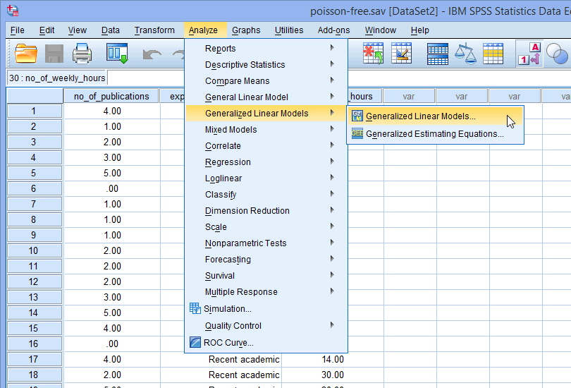
- Click Analyze > Generalized Linear Models > Generalized Linear Models... on the main menu, as shown below:

Published with written permission from SPSS Statistics, IBM Corporation.
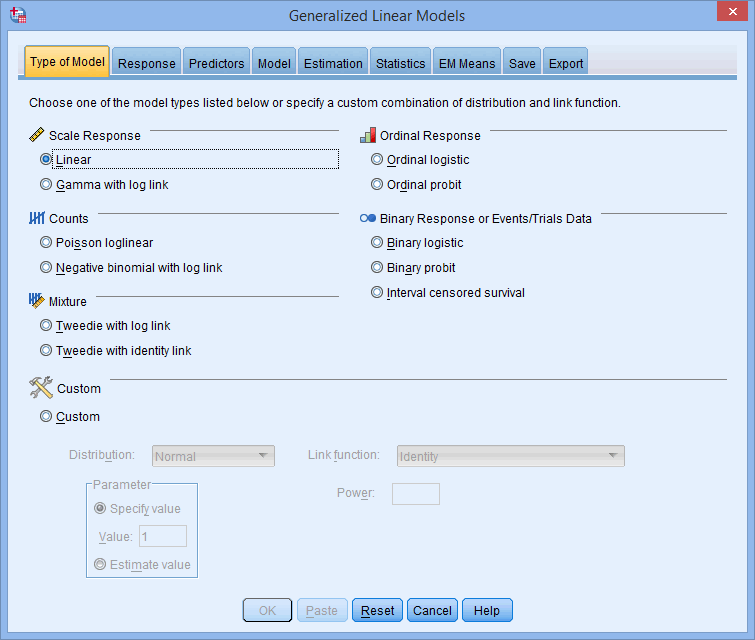
You will be presented with the Generalized Linear Models dialogue box below:
Published with written permission from SPSS Statistics, IBM Corporation.
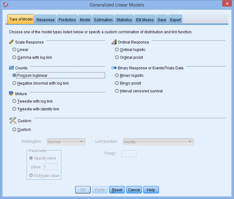
- Select Poisson loglinear in the area, as shown below:
Published with written permission from SPSS Statistics, IBM Corporation.
Note: Whilst it is standard to select Poisson loglinear in the
area in order to carry out a Poisson regression, you can also choose to run a custom Poisson regression by selecting Custom in the area and then specifying the type of Poisson model you want to run using the Distribution:, Link function: and –Parameter– options. - Select the tab. You will be presented with the following dialogue box:
Published with written permission from SPSS Statistics, IBM Corporation.
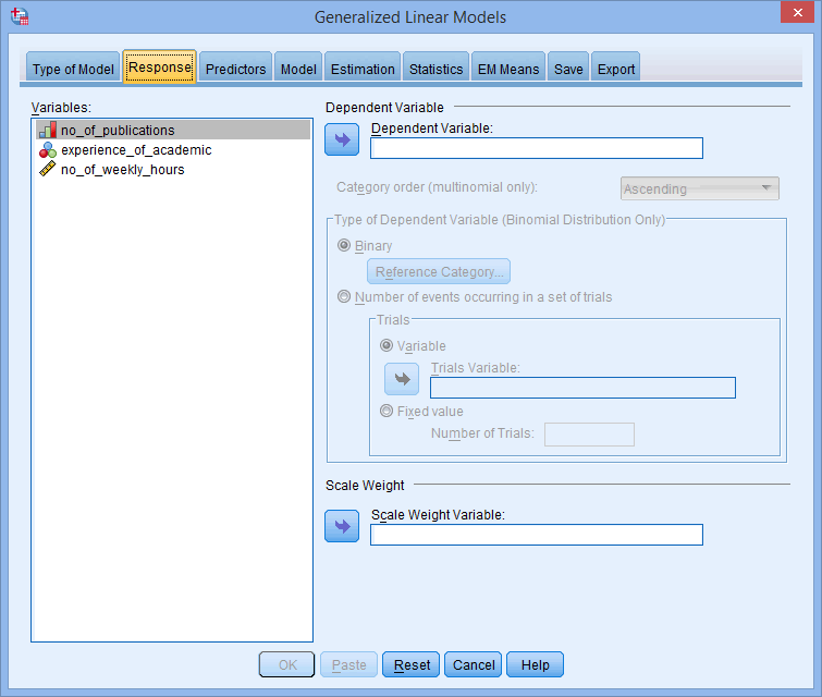
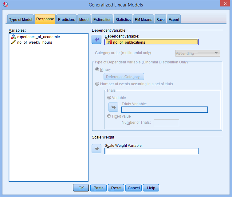
- Transfer your dependent variable, no_of_publications, into the Dependent variable: box in the
 area using the button, as shown below:
Published with written permission from SPSS Statistics, IBM Corporation.
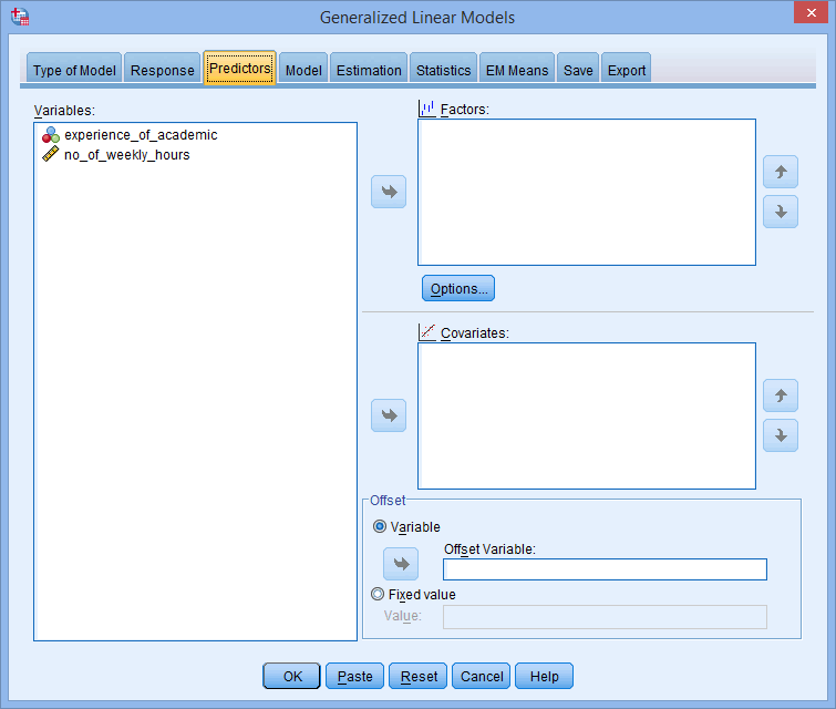
- Select the tab. You will be presented with the following dialogue box:
Published with written permission from SPSS Statistics, IBM Corporation.
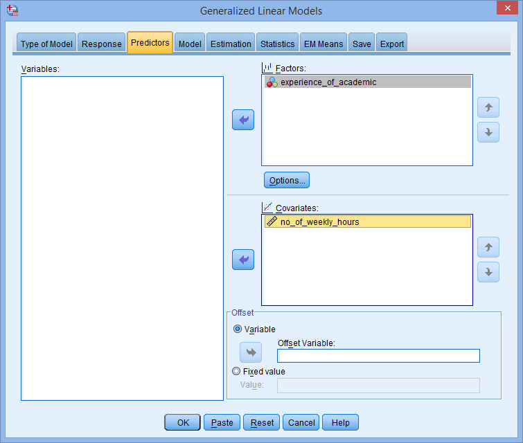
- Transfer the categorical independent variable, experience_of_academic, into the Factors: box and the continuous independent variable, no_of_weekly_hours, into the Covariates: box, using the buttons, as shown below:
Published with written permission from SPSS Statistics, IBM Corporation.
Note 1: If you have ordinal independent variables, you need to decide whether these are to be treated as categorical and entered into the Factors: box, or treated as continuous and entered into the Covariates: box. They cannot be entered into a Poisson regression as ordinal variables.
Note 2: Whilst it is typical to enter continuous independent variables into the Covariates: box, it is possible to enter ordinal independent variables instead. However, if you choose to do this, your ordinal independent variable will be treated as continuous.
Note 3: If you click on the
button the following dialogue box will appear:
In the –Category Order for Factors– area you can choose between the Ascending, Descending and Use data order options. These are useful because SPSS Statistics automatically turns your categorical variables into dummy variables. Unless you are familiar with dummy variables, this can make it a little tricky to interpret the output from a Poisson regression for each of the groups of your categorical variables. Therefore, making changes to the options in the –Category Order for Factors– area can make it easier to interpret your output. - Select the tab. You will be presented with the following dialogue box:
Published with written permission from SPSS Statistics, IBM Corporation.
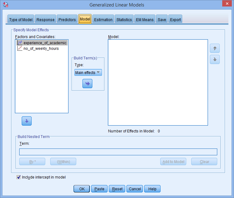
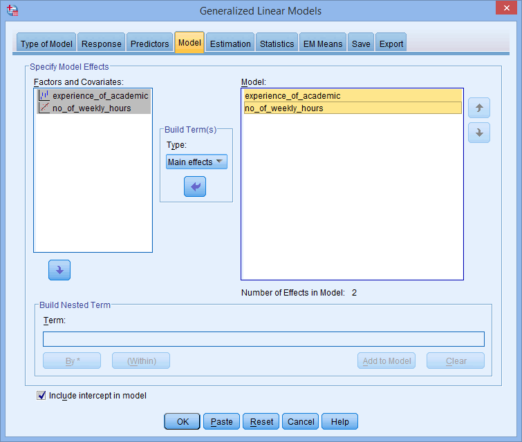
- Keep the default of in the –Build Term(s)– area and transfer the categorical and continuous independent variables, experience_of_academic and no_of_weekly_hours, from the Factors and Covariates: box into the Model: box, using the button, as shown below:
Published with written permission from SPSS Statistics, IBM Corporation.
Note 1: It is in the
dialogue box that you build your Poisson model. In particular, you determine what main effects you have (the option), as well as whether you expect there to be any interactions between your independent variables (the option). If you suspect that you have interactions between your independent variables, including these in your model is important not only to improve the prediction of your model, but also to avoid issues of overdispersion, as highlighted in the Assumptions section earlier.
Whilst we provide an example for a very simply model with just a single main effect (between the categorical and continuous independent variables, experience_of_academic and no_of_weekly_hours), you can easily enter more complex models using the, , . and options in the –Build Term(s)– area depending on the type of main effects and interactions you have in your model.Note 2: You can also build nested terms into your model by adding these into the Term: box in the –Build Nested Term– area. We do not have nested effects in this model, but there are many scenarios where you might have nested terms in your model.
- Select the tab. You will be presented with the following dialogue box:
Published with written permission from SPSS Statistics, IBM Corporation.
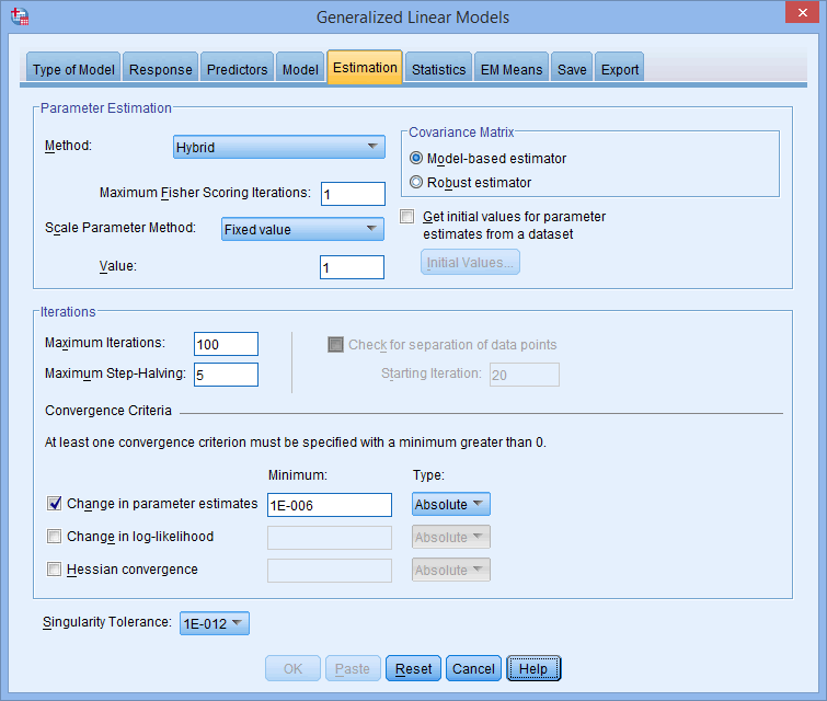
- Keep the default options selected.
Note: There are a number of different options you can select within the –Parameter Estimation– area, including the ability to choose a different: (a) scale parameter method (i.e.,
or instead of in the Scale Parameter Method: box), which might be considered to deal with issues of overdispersion; and (b) covariance matrix (i.e., Robust estimator instead of Model-based estimator in the –Covariance Matrix– area), which presents another potential option (amongst other things) to deal with issues of overdispersion.
There are also a number of specifications you can make in the –Iterations– area in order to deal with issues of non-convergence in your Poisson model. - Select the tab. You will be presented with the following dialogue box:
Published with written permission from SPSS Statistics, IBM Corporation.
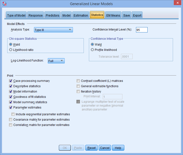
- Select Include exponential parameter estimates in the area, as shown below:
Published with written permission from SPSS Statistics, IBM Corporation.
Note 1: In the
area, you can choose between the Wald and Likelihood ratio based on factors such as sample size and the implications that this can have for the accuracy of statistical significance testing.
In the area, the Lagrange multiplier test can also be useful to determine whether the Poisson model is appropriate for your data (although this cannot be run using the Poisson regression procedure).Note 2: You can also select a wide range of other options from the
and tabs. These include options that are important when examining differences between the groups of your categorical variables as well as testing the assumptions of Poisson regression, as discussed in the Assumptions section earlier. - Click on the button. This will generate the output.


SPSS Statistics
Interpreting the results of a Poisson regression analysis
SPSS Statistics will generate quite a few tables of output for a Poisson regression analysis. In this section, we show you the eight main tables required to understand your results from the Poisson regression procedure, assuming that no assumptions have been violated.
Model and variable information
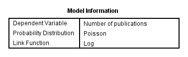
The first table in the output is the Model Information table (as shown below). This confirms that the dependent variable is the "Number of publications", the probability distribution is "Poisson" and the link function is the natural logarithm (i.e., "Log"). If you are running a Poisson regression on your own data the name of the dependent variable will be different, but the probability distribution and link function will be the same.
Published with written permission from SPSS Statistics, IBM Corporation.
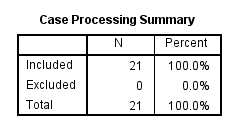
The second table, Case Processing Summary, shows you how many cases (e.g., subjects) were included in your analysis (the "Included" row) and how many were not included (the "Excluded" row), as well as the percentage of both. You can think of the "Excluded" row as indicating cases (e.g., subjects) that had one or more missing values. As you can see below, there were 21 subjects in this analysis with no subjects excluded (i.e., no missing values).
Published with written permission from SPSS Statistics, IBM Corporation.
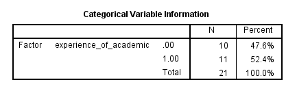
The Categorical Variable Information table highlights the number and percentage of cases (e.g., subjects) in each group of each independent categorical variable in your analysis. In this analysis, there is only one categorical independent variable (also known as a "factor"), which was experience_of_academic. You can see that the groups are fairly balanced in numbers between the two groups (i.e., 10 versus 11). Highly unbalanced group sizes can cause problems with model fit, but we can see that there is no problem here.
Published with written permission from SPSS Statistics, IBM Corporation.
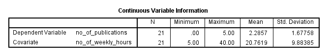
The Continuous Variable Information table can provide a rudimentary check of the data for any problems, but is less useful than other descriptive statistics you can run separately before running the Poisson regression. The best you can get out of this table is to gain an understanding of whether there might be overdispersion in your analysis (i.e., Assumption #5 of Poisson regression). You can do this by considering the ratio of the variance (the square of the "Std. Deviation" column) to the mean (the "Mean" column) for the dependent variable. You can see these figures below:
Published with written permission from SPSS Statistics, IBM Corporation.
The mean is 2.29 and the variance is 2.81 (1.677582), which is a ratio of 2.81 ÷ 2.29 = 1.23. A Poisson distribution assumes a ratio of 1 (i.e., the mean and variance are equal). Therefore, we can see that before we add in any explanatory variables there is a small amount of overdispersion. However, we need to check this assumption when all the independent variables have been added to the Poisson regression. This is discussed in the next section.
Determining how well the model fits
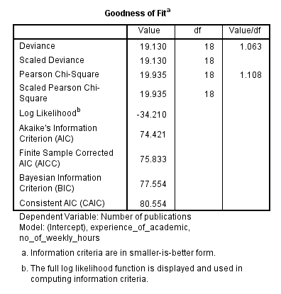
The Goodness of Fit table provides many measures that can be used to assess how well the model fits. However, we will concentrate on the value in the "Value/df" column for the "Pearson Chi-Square" row, which is 1.108 in this example, as shown below:
Published with written permission from SPSS Statistics, IBM Corporation.
A value of 1 indicates equidispersion whereas values greater than 1 indicate overdispersion and values below 1 indicate underdispersion. The most common type of violation of the assumption of equidispersion is overdispersion. With such a small sample size in this example a value of 1.108 is unlikely to be a serious violation of this assumption.
The Omnibus Test table fits somewhere between this section and the next. It is a likelihood ratio test of whether all the independent variables collectively improve the model over the intercept-only model (i.e., with no independent variables added). Having all the independent variables in our example model we have a p-value of .006 (i.e., p = .006), indicating a statistically significant overall model, as shown below in the "Sig." column:
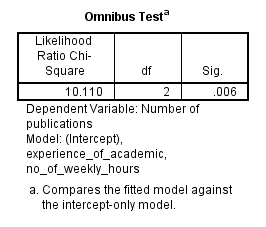
Published with written permission from SPSS Statistics, IBM Corporation.
Now that you know that the addition of all the independent variables generates a statistically significant model, you will want to know which specific independent variables are statistically significant. This is discussed in the next section.
Model effects and statistical significance of the independent variables
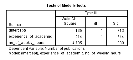
The Tests of Model Effects table (as shown below) displays the statistical significance of each of the independent variables in the "Sig." column:
Published with written permission from SPSS Statistics, IBM Corporation.
There is not usually any interest in the model intercept. However, we can see that the experience of the academic was not statistically significant (p = .644), but the number of hours worked per week was statistically significant (p = .030). This table is mostly useful for categorical independent variables because it is the only table that considers the overall effect of a categorical variable, unlike the Parameter Estimates table, as shown below:
Published with written permission from SPSS Statistics, IBM Corporation.
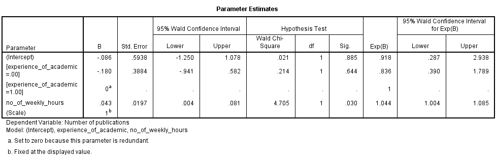
This table provides both the coefficient estimates (the "B" column) of the Poisson regression and the exponentiated values of the coefficients (the "Exp(B)" column). It is usually the latter that are more informative. These exponentiated values can be interpreted in more than one way and we will show you one way in this guide. Consider, for example, the number of hours worked weekly (i.e., the "no_of_weekly_hours" row). The exponentiated value is 1.044. This means that the number of publications (i.e., the count of the dependent variable) will be 1.044 times greater for each extra hour worked per week. Another way of saying this is that there is a 4.4% increase in the number of publications for each extra hour worked per week. A similar interpretation can be made for the categorical variable.
SPSS Statistics
Reporting the results of a Poisson regression analysis
You could write up the results of the number of hours worked per week as follows:
- General
A Poisson regression was run to predict the number of publications an academic publishes in the last 12 months based on the experience of the academic and the number of hours an academic spends each week working on research. For every extra hour worked per week on research, 1.044 (95% CI, 1.004 to 1.085) times more publications were published, a statistically significant result, p = .030.