Multinomial Logistic Regression using SPSS Statistics
Introduction
Multinomial logistic regression (often just called "multinomial regression") is used to predict a nominal dependent variable given one or more independent variables. It is sometimes considered an extension of binomial logistic regression to allow for a dependent variable with more than two categories. As with other types of regression, multinomial logistic regression can have nominal and/or continuous independent variables and can have interactions between independent variables to predict the dependent variable.
For example, you could use multinomial logistic regression to understand which type of drink consumers prefer based on location in the UK and age (i.e., the dependent variable would be "type of drink", with four categories – Coffee, Soft Drink, Tea and Water – and your independent variables would be the nominal variable, "location in UK", assessed using three categories – London, South UK and North UK – and the continuous variable, "age", measured in years). Alternately, you could use multinomial logistic regression to understand whether factors such as employment duration within the firm, total employment duration, qualifications and gender affect a person's job position (i.e., the dependent variable would be "job position", with three categories – junior management, middle management and senior management – and the independent variables would be the continuous variables, "employment duration within the firm" and "total employment duration", both measured in years, the nominal variables, "qualifications", with four categories – no degree, undergraduate degree, master's degree and PhD – "gender", which has two categories: "males" and "females").
This "quick start" guide shows you how to carry out a multinomial logistic regression using SPSS Statistics and explain some of the tables that are generated by SPSS Statistics. However, before we introduce you to this procedure, you need to understand the different assumptions that your data must meet in order for a multinomial logistic regression to give you a valid result. We discuss these assumptions next.
Note: We do not currently have a premium version of this guide in the subscription part of our website. If you would like us to add a premium version of this guide, please contact us.
SPSS Statistics
Assumptions of a multinomial logistic regression
When you choose to analyse your data using multinomial logistic regression, part of the process involves checking to make sure that the data you want to analyse can actually be analysed using multinomial logistic regression. You need to do this because it is only appropriate to use multinomial logistic regression if your data "passes" six assumptions that are required for multinomial logistic regression to give you a valid result. In practice, checking for these six assumptions just adds a little bit more time to your analysis, requiring you to click a few more buttons in SPSS Statistics when performing your analysis, as well as think a little bit more about your data, but it is not a difficult task.
Before we introduce you to these six assumptions, do not be surprised if, when analysing your own data using SPSS Statistics, one or more of these assumptions is violated (i.e., not met). This is not uncommon when working with real-world data rather than textbook examples, which often only show you how to carry out a multinomial logistic regression when everything goes well! However, don’t worry. Even when your data fails certain assumptions, there is often a solution to overcome this. First, let's take a look at these six assumptions:
- Assumption #1: Your dependent variable should be measured at the nominal level. Examples of nominal variables include ethnicity (e.g., with three categories: Caucasian, African American and Hispanic), transport type (e.g., with four categories: bus, car, tram and train), profession (e.g., with five groups: surgeon, doctor, nurse, dentist, therapist), and so forth. Multinomial logistic regression can also be used for ordinal variables, but you might consider running an ordinal logistic regression instead. You can learn more about types of variables in our article: Types of Variable.
- Assumption #2: You have one or more independent variables that are continuous, ordinal or nominal (including dichotomous variables). However, ordinal independent variables must be treated as being either continuous or categorical. They cannot be treated as ordinal variables when running a multinomial logistic regression in SPSS Statistics; something we highlight later in the guide. Examples of continuous variables include age (measured in years), revision time (measured in hours), income (measured in US dollars), intelligence (measured using IQ score), exam performance (measured from 0 to 100), weight (measured in kg), and so forth. Examples of ordinal variables include Likert items (e.g., a 7-point scale from "strongly agree" through to "strongly disagree"), amongst other ways of ranking categories (e.g., a 3-point scale explaining how much a customer liked a product, ranging from "Not very much", to "It is OK", to "Yes, a lot"). Example nominal variables were provided in the previous bullet.
- Assumption #3: You should have independence of observations and the dependent variable should have mutually exclusive and exhaustive categories.
- Assumption #4: There should be no multicollinearity. Multicollinearity occurs when you have two or more independent variables that are highly correlated with each other. This leads to problems with understanding which variable contributes to the explanation of the dependent variable and technical issues in calculating a multinomial logistic regression. Determining whether there is multicollinearity is an important step in multinomial logistic regression. Unfortunately, this is an exhaustive process in SPSS Statistics that requires you to create any dummy variables that are needed and run multiple linear regression procedures.
- Assumption #5: There needs to be a linear relationship between any continuous independent variables and the logit transformation of the dependent variable.
- Assumption #6: There should be no outliers, high leverage values or highly influential points.
You can check assumptions #4, #5 and #6 using SPSS Statistics. Assumptions #1, #2 and #3 should be checked first, before moving onto assumptions #4, #5 and #6. Just remember that if you do not run the statistical tests on these assumptions correctly, the results you get when running a multinomial logistic regression might not be valid.
In the section, Procedure, we illustrate the SPSS Statistics procedure to perform a multinomial logistic regression assuming that no assumptions have been violated. First, we introduce the example that is used in this guide.
SPSS Statistics
Example used in this guide
A researcher wanted to understand whether the political party that a person votes for can be predicted from a belief in whether tax is too high and a person's income (i.e., salary). Therefore, the political party the participants last voted for was recorded in the politics variable and had three options: "Conservatives", "Labour" and "Liberal Democrats". When presented with the statement, "tax is too high in this country", participants had four options of how to respond: "Strongly Disagree", "Disagree", "Agree" or "Strongly Agree" and stored in the variable, tax_too_high. The researcher also asked participants their annual income which was recorded in the income variable. As such, in variable terms, a multinomial logistic regression was run to predict politics from tax_too_high and income.
Note: For those readers that are not familiar with the British political system, we are taking a stereotypical approach to the three major political parties, whereby the Liberal Democrats and Labour are parties in favour of high taxes and the Conservatives are a party favouring lower taxes.
SPSS Statistics
Data setup in SPSS Statistics
In SPSS Statistics, we created three variables: (1) the independent variable, tax_too_high, which has four ordered categories: "Strongly Disagree", "Disagree", "Agree" and "Strongly Agree"; (2) the independent variable, income; and (3) the dependent variable, politics, which has three categories: "Con", "Lab" and "Lib" (i.e., to reflect the Conservatives, Labour and Liberal Democrats).
Note: In the SPSS Statistics procedures you are about to run, you need to separate the variables into covariates and factors. For these particular procedures, SPSS Statistics classifies continuous independent variables as covariates and nominal independent variables as factors. Therefore, the continuous independent variable, income, is considered a covariate. However, where you have an ordinal independent variable, such as in our example (i.e., tax_too_high), you must choose whether to consider this as a covariate or a factor. In our example, it will be treated as a factor.
SPSS Statistics
SPSS Statistics procedure to carry out a multinomial logistic regression
The six steps below show you how to analyse your data using a multinomial logistic regression in SPSS Statistics when none of the six assumptions in the previous section, Assumptions, have been violated. At the end of these six steps, we show you how to interpret the results from your multinomial logistic regression.
Note: The procedure that follows is identical for SPSS Statistics versions 18 to 30, as well as the subscription version of SPSS Statistics, with version 30 and the subscription version being the latest versions of SPSS Statistics. However, in version 27 and the subscription version, SPSS Statistics introduced a new look to their interface called "SPSS Light", replacing the previous look for versions 26 and earlier versions, which was called "SPSS Standard". Therefore, if you have SPSS Statistics versions 27 to 30 (or the subscription version of SPSS Statistics), the images that follow will be light grey rather than blue. However, the procedure is identical.
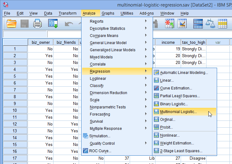
- Click Analyze > Regression > Multinomial Logistic... on the main menu, as shown below:

Published with written permission from SPSS Statistics, IBM Corporation.
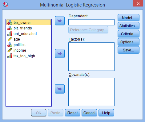
You will be presented with the Multinomial Logistic Regression dialogue box, as shown below:
Published with written permission from SPSS Statistics, IBM Corporation.
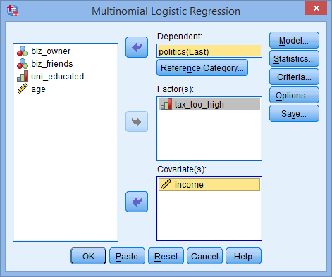
- Transfer the dependent variable, politics, into the Dependent: box, the ordinal variable, tax_too_high, into the Factor(s): box and the covariate variable, income, into the Covariate(s): box, as shown below:
Published with written permission from SPSS Statistics, IBM Corporation.
Note: The default behaviour in SPSS Statistics is for the last category (numerically) to be selected as the reference category. In our example, this is those who voted "Labour" (i.e., the "Labour" category).
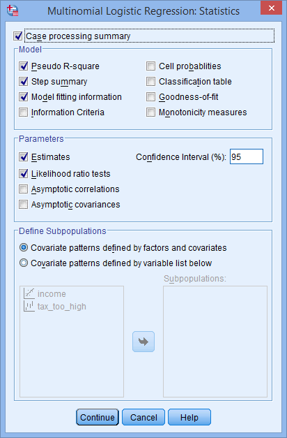
- Click on the button. You will be presented with the Multinomial Logistic Regression: Statistics dialogue box, as shown below:
Published with written permission from SPSS Statistics, IBM Corporation.
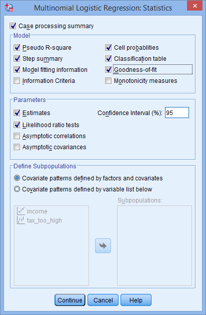
- Click the Cell probabilities, Classification table and Goodness-of-fit checkboxes. You will be presented with the following screenshot:
Published with written permission from SPSS Statistics, IBM Corporation.
- Click on the button and you will be returned to the Multinomial Logistic Regression dialogue box.
- Click on the button. This will generate the results.
SPSS Statistics
Interpreting the results of a multinomial logistic regression
SPSS Statistics will generate quite a few tables of output for a multinomial logistic regression analysis. In this section, we show you some of the tables required to understand your results from the multinomial logistic regression procedure, assuming that no assumptions have been violated.
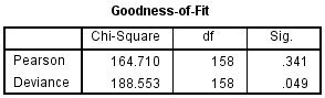
The Goodness-of-Fit table provides two measures that can be used to assess how well the model fits the data, as shown below:
Published with written permission from SPSS Statistics, IBM Corporation.
The first row, labelled "Pearson", presents the Pearson chi-square statistic. Large chi-square values (found under the "Chi-Square" column) indicate a poor fit for the model. A statistically significant result (i.e., p < .05) indicates that the model does not fit the data well. You can see from the table above that the p-value is .341 (i.e., p = .341) (from the "Sig." column) and is, therefore, not statistically significant. Based on this measure, the model fits the data well. The other row of the table (i.e., the "Deviance" row) presents the Deviance chi-square statistic. These two measures of goodness-of-fit might not always give the same result.
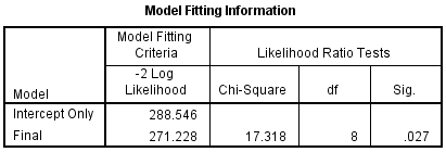
Another option to get an overall measure of your model is to consider the statistics presented in the Model Fitting Information table, as shown below:
Published with written permission from SPSS Statistics, IBM Corporation.
The "Final" row presents information on whether all the coefficients of the model are zero (i.e., whether any of the coefficients are statistically significant). Another way to consider this result is whether the variables you added statistically significantly improve the model compared to the intercept alone (i.e., with no variables added). You can see from the "Sig." column that p = .027, which means that the full model statistically significantly predicts the dependent variable better than the intercept-only model alone.
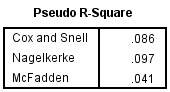
In multinomial logistic regression you can also consider measures that are similar to R2 in ordinary least-squares linear regression, which is the proportion of variance that can be explained by the model. In multinomial logistic regression, however, these are pseudo R2 measures and there is more than one, although none are easily interpretable. Nonetheless, they are calculated and shown below in the Pseudo R-Square table:
Published with written permission from SPSS Statistics, IBM Corporation.
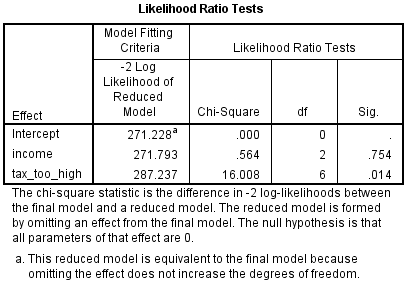
SPSS Statistics calculates the Cox and Snell, Nagelkerke and McFadden pseudo R2 measures. Of much greater importance are the results presented in the Likelihood Ratio Tests table, as shown below:
Published with written permission from SPSS Statistics, IBM Corporation.
This table shows which of your independent variables are statistically significant. You can see that income (the "income" row) was not statistically significant because p = .754 (the "Sig." column). On the other hand, the tax_too_high variable (the "tax_too_high" row) was statistically significant because p = .014. There is not usually any interest in the model intercept (i.e., the "Intercept" row). This table is mostly useful for nominal independent variables because it is the only table that considers the overall effect of a nominal variable, unlike the Parameter Estimates table, as shown below:
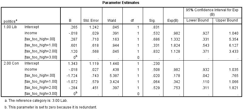
Published with written permission from SPSS Statistics, IBM Corporation.
This table presents the parameter estimates (also known as the coefficients of the model). As you can see, each dummy variable has a coefficient for the tax_too_high variable. However, there is no overall statistical significance value. This was presented in the previous table (i.e., the Likelihood Ratio Tests table). As there were three categories of the dependent variable, you can see that there are two sets of logistic regression coefficients (sometimes called two logits). The first set of coefficients are found in the "Lib" row (representing the comparison of the Liberal Democrats category to the reference category, Labour). The second set of coefficients are found in the "Con" row (this time representing the comparison of the Conservatives category to the reference category, Labour). You can see that "income" for both sets of coefficients is not statistically significant (p = .532 and p = .508, respectively; the "Sig." column).
The only coefficient (the "B" column) that is statistically significant is for the second set of coefficients. It is [tax_too_high=.00] (p = .020), which is a dummy variable representing the comparison between "Strongly Disagree" and "Strongly Agree" to tax being too high. The sign is negative, indicating that if you "strongly agree" compared to "strongly disagree" that tax is too high, you are more likely to be Conservative than Labour. However, because the coefficient does not have a simple interpretation, the exponentiated values of the coefficients (the "Exp(B)" column) are normally considered instead.
SPSS Statistics
Reporting the results of a multinomial logistic regression
You could write up the results of the particular coefficient as discussed above as follows:
It is more likely that you are a Conservative than a Labour voter if you strongly agreed rather than strongly disagreed with the statement that tax is too high.