Independent-samples t-test using SPSS Statistics
Introduction
The independent-samples t-test, also known as the independent t-test, independent-measures t-test, between-subjects t-test or unpaired t-test, is used to determine whether there is a difference between two independent, unrelated groups (e.g., undergraduate versus PhD students, athletes given supplement A versus athletes given supplement B, etc.) in terms of the mean of a continuous dependent variable (e.g., first-year salary after graduation in US dollars, time to complete a 100 meter sprint in seconds, etc.) in the population (e.g., the population of all undergraduate and PhD students in the United States, the population of all sprinters who have competed in an internationally-recognised 100 meter sprint event for their country in the last 12 months, etc.).
For example, you could use an independent-samples t-test to understand whether the mean (average) number of hours students spend revising for exams in their first year of university differs based on gender. Here, the dependent variable is "mean revision time", measured in hours, and the independent variable is "gender", which has two groups: "males" and "females". Alternatively, you could use an independent-samples t-test to understand whether there is a mean (average) difference in weight loss between obese patients who undergo a 12-week exercise programme compared to obese patients who are given dieting pills (appetite suppressors) by their doctor. Here, the dependent variable is "weight loss", measured in kilograms (kg), and the independent variable is "type of weight loss intervention", which has two groups: "exercise programme" and "dieting pills".
In this introductory guide to the independent-samples t-test, we first describe two study designs where the independent-samples t-test is most often used, before explaining why an independent-samples t-test is being carried out to analyse your data rather than simply using descriptive statistics. Next, we set out the basic requirements and assumptions of the independent-samples t-test, which your study design and data must meet. Making sure that your study design, variables and data pass/meet these assumptions is critical because if they do not, the independent-samples t-test is likely to be the incorrect statistical test to use. In the third section of this introductory guide, we set out the example we use to illustrate how to carry out an independent-samples t-test using SPSS Statistics, before showing how to set up your data in the Variable View and Data View of SPSS Statistics. In the Procedure section, we set out the simple 8-step procedure in SPSS Statistics to carry out an independent-samples t-test, including useful descriptive statistics. Next, we explain how to interpret the main results of the independent-samples t-test where you will determine whether there is a statistically significant mean difference between your two groups in terms of the dependent variable, as well as a 95% confidence interval (CI) of the mean difference. We also introduce the importance of calculating an effect size for your results. In the final section, Reporting, we explain the information you should include when reporting your results. A Bibliography and Referencing section is included at the end for further reading. Therefore, to continue with this introductory guide, go to the next section.
SPSS Statistics
Study designs where an independent-samples t-test could be used
An independent-samples t-test is most often used to analyse the results of two different types of study design: (a) determining if there is a mean difference between two independent groups; and (b) determining if there is a mean difference between two interventions. To learn more about these two types of study design where the independent-samples t-test can be used, see the examples below:
Note 1: An independent-samples t-test can also be used to determine if there is a mean difference between two change scores (also known as gain scores). However, a one-way ANCOVA is more commonly recommended for this type of study design.
Note 2: In the examples that follow we introduce terms such as mean difference, 95% CI of the mean difference, statistical significance value (i.e., p-value), and effect size. However, do not worry if you do not understand these terms. They will become clearer as you work through this introductory guide.
- Difference between two INDEPENDENT GROUPS
- Difference between two TREATMENT/EXPERIMENTAL GROUPS
Difference between two INDEPENDENT GROUPS
Some degree courses include mandatory 1-year internships (also known as placements), which are thought to help students’ job prospects after graduating. Therefore, imagine that a researcher wanted to determine whether students who enrolled in a 3-year degree course that included a mandatory 1-year internship (also known as a placement) received better graduate salaries than students who did not undertake an internship. The researcher was specifically interested in students who undertook a Finance degree.
A total of 60 first-year graduates who had undertaken a Finance degree were recruited to the study. Of these 60 graduates, 30 had undertaken a 3-year Finance degree that included a mandatory 1-year internship. This group of 300 graduates represented the "internship group". The other 30 had undertaken a 3-year Finance degree that did not include an internship. This group of 30 graduates represented the "no internship group". The first-year graduate salaries of all 60 graduates were recorded in US dollars.
Therefore, in this study the dependent variable was "salary", measured in US dollars, and the independent variable was "course type", which had two independent groups: "internship group" and "no internship group". The two groups were independent because no graduate could be in more than one group and the students in the two groups could not influence each other’s salaries.
The researcher analysed the data collected to determine whether salaries were greater (or smaller) in the internship group compared to the no internship group. An independent-samples t-test was used to determine whether there was a statistically significant mean difference in the salaries between the internship group and the no internship group. The 95% confidence interval (CI) of the mean difference was included as part of the analysis to improve our assessment of the independent-samples t-test result. The independent-samples t-test was supplemented with an effect size calculation to assess the practical/clinical importance of the mean difference in salaries between the internship group and the no internship group. Together, the mean difference, 95% CI of the mean difference, statistical significance value (i.e., p-value), and effect size calculation are used to determine whether students who enrolled in a 3-year degree course that included a mandatory 1-year internship (also known as a placement) received better graduate salaries than students who did not undertake an internship.
Difference between two TREATMENT/EXPERIMENTAL GROUPS
Some parents use financial rewards (i.e., money) as an incentive to encourage their children to get top marks in their exams (e.g., an "A" grade or what might be a score of 80 or more out of 100). Therefore, imagine that an educational psychologist wanted to determine whether financial rewards increased academic performance amongst school children.
A total of 26 students were randomly assigned to one of two groups. In one group, the school children were offered $500 if they got an "A" grade in their maths exam. This is called the "experimental group". In the other group, the school children are not offered anything, irrespective of how well they performed in the same maths exam. This is called the "control group". All 26 students undertook the same maths exam. After the students have taken the maths exam, their scores (between 0 and 100 marks) were recorded.
Therefore, in this study the dependent variable was "exam result", measured from 0 to 100 marks, and the independent variable was "financial reward", which had two independent groups: "experimental group" and "control group". The two groups were independent because no student could be in more than one group and the students in the two groups were unable to influence each other’s exam results.
The researcher analysed the data collected to determine whether the exam results were better (or worse) amongst students in the experimental group compared to the control group. An independent-samples t-test was used to determine whether there was a statistically significant mean difference in the exam results between the experimental group and the control group. The 95% confidence interval (CI) of the mean difference was included as part of the analysis to improve our assessment of the independent-samples t-test result. The independent-samples t-test was supplemented with an effect size calculation to assess the practical/clinical importance of the mean difference in exam results between the experimental group and the control group. Together, the mean difference, 95% CI of the mean difference, statistical significance value (i.e., p-value), and effect size calculation are used to determine whether financial rewards increased academic performance amongst school children.
In the next section we explain why you are using an independent-samples t-test to analyse your results, rather than simply using descriptive statistics.
SPSS Statistics
Understanding why the independent-samples t-test is being used
To briefly recap, an independent-samples t-test is used to determine whether there is a difference between two independent, unrelated groups (e.g., undergraduate versus PhD students, athletes given supplement A versus athletes given supplement B, etc.) in terms of the mean of a continuous dependent variable (e.g., first-year salary after graduation in US dollars, time to complete a 100 meter sprint in seconds, etc.) in the population (e.g., the population of all PhD students in the United States, the population of all sprinters who have competed in an internationally-recognised 100 meter sprint event for their country in the last 12 months, etc.).
In other words, you are using an independent-samples t-test because you are not only interested in determining whether there is a mean difference in the dependent variable between your two groups in your single study (i.e., the sample of 150 male students and sample of 150 female students), but whether there is a mean difference in these two samples in the wider populations from which these two samples were drawn. To understand these two concepts – sample versus population – and how the independent-samples t-test is used to make inferences from a sample to a population, imagine a study where a researcher wanted to know if there was a mean difference in the amount of time male and female university students in the United States use their mobile phones each week. In this example, the dependent variable is "weekly screen time" and the two independent groups are "male" and "female" university students in the United States.
Ideally, we would test the whole population of university students in the United States to determine if there were differences in weekly screen time between males and females. We could then simply compare the mean difference in weekly screen time between all male and all female students using descriptive statistics to understand whether there was a difference. However, it is rarely possible to study the whole population (i.e., imagine the time and cost involved in collecting data on weekly screen time for the millions of university students in the United States). Since we cannot test everyone, we use a sample, which is a subset of the population. In order to make inferences from a sample to a population, we try to obtain a sample that is representative of the population we are studying. Here, the term "inferences" simply means that we are trying to make predictions/statements about a population using data from a sample that has been drawn from that population.
For example, imagine that we randomly selected 150 male and 150 female university students in the United States to form our two samples. After recording the weekly screen time of these 300 students over a 3-month period, we found that female students spent 27 minutes more time viewing their mobile phones each week compared to male students. Therefore, 27 minutes is the mean difference in weekly screen time between male and female university students in our two samples. This sample mean difference, which is called a "point estimate", is the best estimate that we have of what the population mean difference is (i.e., what the mean difference in weekly screen time is between all male and females university students in the United States, which is the population being studied).
We use this sample mean difference to estimate the population mean difference. However, the mean difference of 27 minutes in weekly screen time between males and females is based on only a single study of one sample of 150 male students and another sample of 150 female students, and not from the millions of university students in the United States. If we carried out a second study with a sample of 150 male students and a sample of 150 female students, or a third study with a sample of 150 male students and a sample of 150 female students, or a fourth study with a sample of 150 male students and a sample of 150 female students, it is likely that the mean difference in weekly screen time will be different each time, or at least, most of the time (e.g., 31 minutes in the second study, 25 minutes in the third study, 28 minutes in the fourth study). In other words, there will be some variation in the sample mean difference each time we sample our populations.
As previously stated, the sample mean difference is the best estimate of the population mean difference, but since we have just one study where we took a single sample from each of our two populations, we know that this estimate of the population mean difference in weekly screen time between male and female students will vary (i.e., it will not always be the same as in this study). In order to quantify this uncertainty in our estimate of the population mean difference, we can use the independent-samples t-test to provide a 95% confidence interval (CI), which is a way of providing a measure of this uncertainty. Presenting a mean difference with a 95% CI to understand what the population mean difference is, and your uncertainty in its value, is an approach called "estimation". Another approach uses a null hypothesis and p-value and is called significance testing or Null Hypothesis Significance Testing (NHST). It is important that you understand both approaches when analysing your data using an independent-samples t-test because they affect how you: (a) carry out an independent-samples t-test using SPSS Statistics, as discussed in the Procedure section later; and (b) interpret and report your results, as discussed in the Interpreting Results and Reporting sections respectively. In fact, it is being more common practice to report both p-values and confidence intervals (CI) in journal articles and student reports (e.g., dissertations/theses). Therefore, both approaches are briefly discussed below:
- Estimation using confidence intervals (CI): One approach to quantify the uncertainty in using the sample mean difference to estimate the population mean difference is to use a confidence interval (CI). When doing so, you can set different levels of confidence for your confidence interval (CI). For example, the most common confidence interval (CI) is the 95% CI, which is the default in SPSS Statistics (and most statistics packages). Therefore, we show you how to select the 95% CI using SPSS Statistics in the Procedure section later.
A confidence interval will give you, based on your sample data, a likely/plausible range of values that the mean difference might be in the population. For example, we know that the mean difference in weekly screen time between male and female students in our two samples was 27 minutes. A 95% CI could suggest that the mean difference in weekly screen time between male and female students in the population might plausibly be somewhere between 13 minutes and 42 minutes. Here, 13 minutes reflects the lower bound of the 95% CI and 42 minutes reflect the upper bound of the 95% CI, both of which are reported by SPSS Statistics when you carry out an independent-samples t-test.
The 95% CI is a very useful method to quantify the uncertainty in using the sample mean difference to estimate the population mean difference because although the sample mean difference is the best estimate that you have of the population mean difference, in reality, the mean difference in the population could plausibly be any value between the lower bound and upper bound of the 95% CI.
If you choose to increase the CI when carrying out an independent-samples t-test from, for example, 95% to 99%, you increase your level of confidence that the population mean difference is somewhere between the lower and upper bounds that are reported.
- Null Hypothesis Significance Testing (NHST) using p-values: Another approach to statistical inference is to test your sample data against a null hypothesis in a process called Null Hypothesis Significance Testing (NHST). NHST is used as a means to find evidence against a null hypothesis. The null hypothesis most commonly tested when carrying out an independent-sample t-test is that there is no mean difference between two groups in the population. The p-value calculated as part of NHST is the probability of finding a result as extreme or more extreme than the result in your study, given that the null hypothesis is true. If your result – or one more extreme – is unlikely to have happened by chance (i.e., due to sampling variation), you make the declaration that you believe the null hypothesis is false (i.e., there is a mean difference between the two groups in the population). NHST does not say what this difference might be. Whether to accept or reject that there is a difference in the population is based on a preset probability level.
Note: Unless you are familiar with statistics, the idea of NHST can be a little challenging at first and benefits from a detailed description, but we will try to give a brief overview in this section. However, since it can be challenging to understand how the independent-samples t-test is used under NHST, we will be adding a guide dedicated to explaining this, including concepts such as the t-distribution, alpha (ɑ) levels, statistical power, Type I and Type II errors, p-values, and more. If you would like us to let you know when we add this guide to the site, please contact us.
Under NHST, the independent-samples t-test is used to test the null hypothesis that there is no mean difference between your two groups in the population, based on the data from your two samples. For example, it tests the null hypothesis that there is no mean difference in weekly screen time between male and female students in the population. Furthermore, the independent-samples t-test is typically used to test the null hypothesis that the mean difference between the two groups in the population is zero (e.g., a mean difference of 0 minutes of weekly screen time between female and female students), which is also referred to as the nil hypothesis, but it can be tested against a specific value (e.g., a mean difference of 20 minutes of weekly screen time between male and female students). Whilst the null hypothesis states that there is no mean difference between your two groups in the population, the alternative hypothesis states that there is a mean difference between your two groups in the population (e.g., the alternative hypothesis that the mean difference in weekly screen time between male and female students is not 0 minutes or the specific value you set, such as 20 minutes, in the population).
Determining whether to reject or fail to reject the null hypothesis is based on a preset probability level (i.e., sometimes called an alpha (ɑ) level). This alpha (ɑ) level is usually set at .05, which means that if the p-value is less than .05 (i.e., p < .05), you declare the result to be statistically significant, such that you reject the null hypothesis and accept the alternative hypothesis. Alternatively, if the p-value is greater than .05 (i.e., p > .05), you declare the result to be not statistically significant, such that you fail to reject the null hypothesis and reject the alternative hypothesis.
These concepts can be fairly difficult to understand without further explanation, but for the purpose of this introductory guide, the important point is that the independent-samples t-test will produce a p-value that can be used to either (a) reject the null hypothesis of no mean difference in the population and accept the alternative hypothesis that there is a mean difference; or (b) fail to reject the null hypothesis, suggesting that there is not enough evidence to accept the alternative hypothesis that there is a mean difference in the population (i.e., rejecting the alternative hypothesis that there is a mean difference). It is important to note that you cannot accept the null hypothesis that there is no mean difference.
A major criticism of NHST is that it results in a dichotomous decision where you simply conclude that there either is a mean difference between your two groups in the population or there is not a mean difference. Therefore, it provides far less information that the 95% CI, which is now the preferred approach. Nonetheless, when carrying out an independent-samples t-test, it is common to interpret and report both the p-value and 95% CI.
Hopefully this section has highlighted how: (a) the independent-samples t-test, using the NHST approach, gives you an idea of whether there is a mean difference between your two groups in the population, based on your sample data; and (b) the independent-samples t-test, as a method of estimation using confidence intervals (CI), provides a plausible range of values that the mean difference between your two groups could be in the population, based on your sample data. In order that these p-values and confidence intervals (CI) are accurate/valid, your sample data must "pass/meet" a number of basic requirements and assumptions of the independent-samples t-test. This is discussed in the next section: Basic requirements and assumptions of the independent-samples t-test.
SPSS Statistics
Basic requirements and assumptions of the independent-samples t-test
The first and most important step in an independent-samples t-test analysis is to check whether it is appropriate to use this statistical test. After all, the independent-samples t-test will only give you valid/accurate results if your study design and data "pass/meet" six assumptions that underpin the independent-samples t-test.
In many cases, the independent-samples t-test will be the incorrect statistical test to use because your data "violates/does not meet" one or more of these assumptions. This is not uncommon when working with real-world data, which is often "messy", as opposed to textbook examples. However, there is often a solution, whether this involves using a different statistical test, or making adjustments to your data so that you can continue to use an independent-samples t-test.
Before discussing these options further, we briefly set out the six assumptions of the independent-samples t-test, three of which relate to your study design and how you measured your variables (i.e., Assumptions #1, #2 and #3 below), and three which relate to the characteristics of your data (i.e., Assumptions #4, #5 and #6 below):
- Assumption #1: You have one dependent variable that is measured on a continuous scale (i.e., it is measured at the interval or ratio level). Examples of continuous variables include salary (measured in US dollars), revision time (measured in hours), height (measured in cm), test score (measured from 0 to 100), intelligence (measured using IQ score), age (measured in years), and so forth.
- Assumption #2: You have one independent variable that consists of two categorical, independent groups (i.e., you have a dichotomous variable). A dichotomous variable can be either ordinal or nominal. Ordinal variables with two groups, also referred to as levels, include income level (two levels: "low income" and "high income"), exam result (two levels: "pass" and "fail"), intelligence (two levels: "below average IQ" and "above average IQ"), age group (two levels: "under 21 years old" and "21 years old and over"), educational level (two levels: "undergraduate" and "postgraduate"), and so forth. Nominal variables with two groups include gender (two groups: "male" and "female"), drug trial (two groups: "drug A" and "drug B"), choice of transport (two groups: "car" and "bus"), employment status (two groups: "employed" and "unemployed"), credit card application (two groups: "granted" and "denied"), presence of heart disease (two groups: "yes" and "no"), and so forth.
Note: You can learn more about the differences between dependent and independent variables, as well as continuous, ordinal, nominal and dichotomous variables in our guide: Types of variable.
- Assumption #3: There should be independence of observations, which means that there is no relationship between the observations in each group of the independent variable or between the groups themselves. Indeed, an important distinction is made in statistics when comparing values from either different individuals or from the same individuals. Independent groups (in an independent-samples t-test) are groups where there is no relationship between the participants in either of the groups. Most often, this occurs simply by having different participants in each group.
For example, if you split a group of individuals into two groups based on their gender (i.e., a male group and a female group), no one in the female group can be in the male group and vice versa. As another example, you might randomly assign participants to either a control trial or an intervention trial. Again, no participant can be in both the control group and the intervention group. This will be true of any two independent groups you form (i.e., a participant cannot be a member of both groups). In actual fact, the "no relationship" part extends a little further and requires that participants in both groups are considered unrelated, not just different people; for example, participants might be considered related if they are husband and wife, or twins. Furthermore, participants in Group A cannot influence any of the participants in Group B, and vice versa.
If you are using the same participants in each group, or they are otherwise related, a dependent t-test (also known as a paired-samples t-test) is a more appropriate test. An example of where related observations might be a problem is if all the participants in your study (or the participants within each group) were assessed together, such that a participant's performance affects another participant's performance (e.g., participants encourage each other to lose more weight in a 'weight loss intervention' when assessed as a group compared to being assessed individually; or athletic participants being asked to complete '100m sprint tests' together rather than individually, with the added competition amongst participants resulting in faster times, etc.).
Independence of observations is largely a study design issue rather than something you can test for, but it is an important assumption of the independent-samples t-test. If your study fails this assumption, you will need to use another statistical test instead of the independent-samples t-test.
Since assumptions #1, #2 and #3 relate to your study design and how you measured your variables, if any of these three assumptions are not met (i.e., if any of these assumptions do not fit with your research), the independent-samples t-test is the incorrect statistical test to analyse your data. It is likely that there will be other statistical tests you can use instead, but the independent-samples t-test is not the correct test.
After checking if your study design and variables meet assumptions #1, #2 and #3, you should now check if your data also meets assumptions #4, #5 and #6 below. When checking if your data meets these three assumptions, do not be surprised if this process takes up the majority of the time you dedicate to carrying out your analysis. As we mentioned above, it is not uncommon for one or more of these assumptions to be violated (i.e., not met) when working with real-world data rather than textbook examples. However, with the right guidance this does not need to be a difficult process and there are often other statistical analysis techniques that you can carry out that will allow you to continue with your analysis.
- Assumption #4: There should be no problematic outliers in your data. An outlier is a single case/observation in your data set that does not follow the usual pattern. For example, imagine a study comparing income levels between male and female graduates in full-time employment in the United Kingdom in their first year after leaving university. Of the 60 graduates in the study, salaries ranged between £16,000 and £48,000, except for one graduate who earnt more than £1,500,000 (e.g., she had started a tech firm at university and sold a stake in this during her first year after graduation; or he was working for his father’s family business who could afford to pay an extremely high salary that was not linked to his work at the business). In the event, you would be unlikely to know the reason why the graduate earnt more than £1,500,000, only that this salary does not fit the unusual pattern of salaries amongst the sample of 60 graduates in the study (and most likely not the wider population of first year graduates). When using an independent-samples t-test, this might be considered an outlier.
Strictly speaking, testing for outliers is not an assumption of the independent-samples t-test. However, outliers can be problematic because they can disproportionately influence the assumptions and result of the independent-samples t-test, and lead to invalid conclusions. Therefore, you need to detect if there are any problematic outliers in your data before running an independent-samples t-test. Fortunately, there are several methods to detect outliers using SPSS Statistics, as well as methods to deal with outliers when you have any in your data. Ways to deal with outliers range from applying transformations to your data to techniques such as winsorization, which can help you to overcome problems associated with having outliers in your data and allow you to continue with your analysis.
Note: Outliers are not inherently "bad" (i.e., an outlier is not bad simply because it is an outlier). Therefore, when deciding how to deal with outliers in your data, you not only need to consider the statistical implications of any outliers, but also theoretical factors that relate to your research goals and study design.
- Assumption #5: Your dependent variable should be approximately normally distributed for each category of your independent variable. In other words, the distribution of scores of your dependent variable should approximately follow a normal distribution in each category of your independent variable. Taking the example of male and female first-year graduate salaries above, the distribution of graduate salaries should be approximately normally distributed for "males" and approximately normally distributed for "females". Therefore, before you run an independent-samples t-test, you need to check whether these two groups are approximately normally distributed using a mix of numeric methods (e.g., the Shapiro-Wilk test of normality) and graphical methods (e.g., histograms and Normal Q-Q plots), all of which can be carried out using SPSS Statistics. If your data is not normally distributed there are methods to deal with non-normality (e.g., applying a transformation to your data), and after applying these methods, it may still be possible to use an independent-samples t-test. If your data is not normally distributed and no methods are able to "coax" your data towards normality, the independent-samples t-test may be the incorrect statistical test to analyse your data (although there are some exceptions to this). However, there are other statistical tests that can be used when your data violates the assumption of normality.
Note: Technically, it is the residuals that must be approximately normally distributed within each group rather than the data within each group, but in an independent-samples t-test, the results will be the same.
- Assumption #6: There needs to be homogeneity of variances, which means that the (population) variance for each category of your independent variable is the same. You can test whether your data meets this assumption using SPSS Statistics using Levene's test for homogeneity of variances. If your data does not meet this assumption, the independent-samples t-test is not a suitable statistical test. However, you can run a different t-test instead, known as the Welch t-test, which makes an adjustment for unequal variances. The Welch t-test can also be run using SPSS Statistics.
Therefore, before running an independent-samples t-test it is critical that you first check whether your data meets assumption #4 (i.e., no problematic outliers), assumption #5 (i.e., normality) and assumption #6 (i.e., homogeneity of variances). In some cases, failure to meet one or more of these assumptions will make the independent-samples t-test the incorrect statistical test to use. In other cases, you may simply have to make some adjustments to your data before continuing to analyse it using an independent-samples t-test.
Due to the importance of checking that your data meets assumptions #4, #5 and #6, we dedicate seven pages of our enhanced independent t-test guide to help you get this right. This includes: (1) setting out the procedures in SPSS Statistics to test these assumptions; (2) explaining how to interpret the SPSS Statistics output to determine if you have met or violated these assumptions; and (3) explaining what options you have if your data does violate one or more of these assumptions. You can access this enhanced guide by subscribing to Laerd Statistics, which will also give you access to all of the enhanced guides in our site.
When you are confident that your data has met all six assumptions described above, you can carry out an independent-samples t-test to determine whether there is a difference between the two groups of your independent variable in terms of the mean of your dependent variable. In the sections that follow we show you how to do this using SPSS Statistics, based on the example we set out in the next section: Example used in this guide.
SPSS Statistics
Example used in this guide
A researcher wanted to know whether exercise or diet is most effective at improving a person’s cardiovascular health. One measure of cardiovascular health is the concentration of cholesterol in the blood, measured in mmol/L, where lower cholesterol concentrations are associated with improved cardiovascular health. For example, a cholesterol concentration of 3.57 mmol/L would be associated with better cardiovascular health compared to a cholesterol concentration of 6.04 mmol/L.
Being overweight and/or physically inactive increases the concentration of cholesterol in your blood. Both exercise and weight loss can reduce cholesterol concentration. However, imagine that it is not known whether exercise or weight loss through dieting is most effective for lowering blood cholesterol concentration. Therefore, a researcher decided to investigate whether an exercise or dietary intervention was more effective in lowering cholesterol levels.
In this fictitious study, the researcher recruited 40 male participants who were classified as being "sedentary" (i.e., they engaged in only a low amount of daily activity and did not exercise). These 40 participants were randomly assigned to one of two groups. One group underwent a dietary intervention where participants took part in a 6-month dietary programme that restricted how much they could eat each day (i.e., determining their daily calorific consumption). This group was called the "diet" group. The other group underwent an exercise intervention where participants took part in a 6-month exercise programme consisting of 4 x 1-hour exercise sessions per week. This experimental group was called the "exercise" group. After 6 months, the cholesterol concentration of participants was measured (in mmol/L) in the diet group and the exercise group.
Note: To ensure that the assumption of independence of observations was met, as discussed earlier, participants could only be in one of these two groups and the two groups did not have any contact with each other.
To determine which intervention – the diet intervention or the exercise intervention – was most effective in improving cardiovascular health (i.e., by lowering participants' cholesterol concentrations), the researcher carried out an independent-samples t-test to:
- (a) determine whether there was a mean difference in cholesterol concentration between the diet group and the exercise group in the population from which the sample of 40 male participants was drawn.
- (b) assess the plausible range of values that the mean difference between the diet group and the exercise group could be in the population, based on the sample of 40 male participants, using the 95% confidence interval (CI) of the mean difference.
Using the results from the independent-samples t-test, the researcher then:
- (c) calculated a standardised effect size, such as Cohen's d (Cohen, 1988). Since we have yet to introduce the idea of effect sizes in this guide, see the explanatory box below:
Explanation: As explain in the earlier section, Understanding why the independent-samples t-test is being used, the independent-samples t-test: (a) using the NHST approach, gives you an idea of whether there is a mean difference between your two groups in the population, based on your sample data; and (b) as a method of estimation using confidence intervals (CI), provides a plausible range of values that the mean difference between your two groups could be in the population, based on your sample data. However, the NHST approach does not indicate the "size" of the mean difference, unlike the estimation approach. Also, neither approach provide a standardised effect size.
As an introduction to effect size measures, these can be classified into two categories: unstandardised and standardised.
An unstandardised effect size is reported using the units of measurement of the dependent variable. In our example, the dependent variable, cholesterol concentration, is being measured using mmol/L. Therefore, imagine that the mean difference in cholesterol concentration between the exercise group and diet group after the 6-month intervention is 0.52 mmol/L. The unstandardised effect size would be 0.52 mmol/L. To take another example we used earlier in this guide, if the mean difference in weekly screen time between male and female university students was 27 minutes, then 27 minutes is the unstandardised effect size (i.e., the dependent variable, weekly screen time, was measured in minutes).
Alternatively, a standardised effect size removes the units of measurement (i.e., they are unitless) due to the standardisation. Therefore, standardised effect sizes are useful when: (a) the units of measurement of the dependent variable are not meaningful/intuitive (e.g., a dependent variable such as job satisfaction, which may be created by totalling or averaging the scores from multiple 5-point Likert item questions in a survey); and/or (b) when you want to compare the "size" of an effect between different studies (e.g., the effect of an exercise and dietary intervention on cholesterol concentration reported in different studies).
There are many different types of standardised effect size, with different types often trying to "capture" the importance of your results in different ways. Unfortunately, SPSS Statistics does not automatically produce a standardised effect size as part of an independent-samples t-test analysis. However, it is easy to calculate a standardised effect size such as Cohen's d (Cohen, 1988) using the results from the independent-samples t-test analysis.
Therefore, in the example we are using to demonstrate an independent-samples t-test in this introductory guide, the continuous dependent variable is Cholesterol and the dichotomous independent variable is the Intervention, which has two groups: "diet" and "exercise". In the next section, we explain how to set up your data in SPSS Statistics to run an independent-samples t-test using these two variables: Cholesterol and Intervention.
SPSS Statistics
Data setup in SPSS Statistics when carrying out an independent-samples t-test
To carry out an independent-samples t-test, you have to set up two variables in SPSS Statistics. In this example, these are:
(1) The dependent variable, Cholesterol, which is cholesterol concentration of participants, measured in mmol/L.
(2) The independent variable, Intervention, which has two groups – "Diet" and "Exercise" – to reflect the 20 participants who underwent the 6-month dietary intervention (i.e., the diet group) and the 20 participants who underwent the 6-month exercise intervention (i.e., the exercise group).
To set up these variables, SPSS Statistics has a Variable View where you define the types of variables you are analysing and a Data View where you enter your data for these variables. First, we show you how to set up your dependent variable and then your independent variable in the Variable View window of SPSS Statistics. Finally, we show you how to enter your data into the Data View window.
The "Variable View" in SPSS Statistics
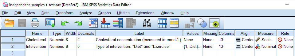
At the end of the data setup process, your Variable View window will look like the one below, which illustrates the setup for both the dependent variable, Cholesterol, and the independent variable, Intervention:

Published with written permission from SPSS Statistics, IBM Corporation.
In the Variable View window above, you will have entered two variables: one on each row. For our example, we have put the continuous dependent variable, Cholesterol, on row , and the dichotomous independent variable, Intervention, on row .
Note: The order that you enter your variables into the Variable View is irrelevant. It will simply determine the order of the columns in the Data View, as explained later.
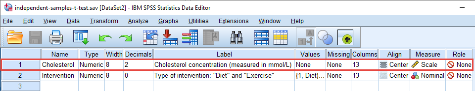
First, look at the continuous dependent variable, Cholesterol, on row below:
Published with written permission from SPSS Statistics, IBM Corporation.
The name of your dependent variable should be entered in the cell under the column (e.g., "Cholesterol" in row to represent our continuous dependent variable, Cholesterol). There are certain "illegal" characters that cannot be entered into the cell. Therefore, if you get an error message and you would like us to add an SPSS Statistics guide to explain what these illegal characters are, please contact us.
Note: For your own clarity, you can also provide a label for your variables in the column. For example, the label we entered for "Cholesterol" was "Cholesterol concentration (measured in mmol/L)".
The cell under the column should show , indicating that you have a continuous dependent variable, whilst the cell under the column should show .
Note: We suggest changing the cell under the column from to , but you do not have to make this change. We suggest that you do because there are certain analyses in SPSS Statistics where the setting results in your variables being automatically transferred into certain fields of the dialogue boxes you are using. Since you may not want to transfer these variables, we suggest changing the setting to so that this does not happen automatically.
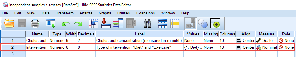
Next, look at the dichotomous independent variable, Intervention, on row below:
Published with written permission from SPSS Statistics, IBM Corporation.
Enter the name of your independent variable in the cell under the column (e.g., "Intervention" in our example). As before, you can also provide a label for your independent variable in the column. For example, the label we entered for "Intervention" was "Type of intervention: "Diet" and "Exercise"".
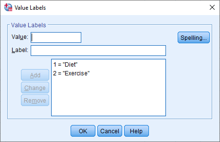
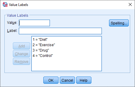
The cell under the column should contain the information about the groups/levels of your independent variables (e.g., "Diet" and "Exercise" for Intervention). To enter this information, click into the cell under the column for your independent variable. The button will appear in the cell. Click on this button and the Value Labels dialogue box will appear. You now need to give each group/level of your independent variable a "value", which you enter into the Value: box (e.g., "1"), as well as a "label", which you enter into the Label: box (e.g., "Diet"). By clicking on the button the coding will appear in the main box (e.g., "1.00 = "Diet" for Intervention). The setup for our independent variable is shown in the Value Labels dialogue box below:
Published with written permission from SPSS Statistics, IBM Corporation.
Note: You will typically enter an integer (e.g., "1") into the Value: box to represent the group/levels of your independent variable and not a decimal (e.g., "1.00"). However, SPSS Statistics adds the 2 decimal places by default when you click on the button (e.g., 1.00 = "Diet"). Therefore, you can simply click into the cells under the column and change these to "0" using the arrows, which is why "Diet" is coded as "1" and not "1.00" in the Value Labels box above. Therefore, do not think that you have done anything wrong if 2 decimals places have been added to the values you set up in the Value Labels box.
The cell under the column should show if you have a nominal independent variable (e.g., Intervention, as in our example) or if you have an ordinal independent variable (e.g., imagine an ordinal variable such as "Body Mass Index" (BMI), BMI, which has four levels: "Underweight", "Normal", "Overweight", and "Obese"). Finally, the cell under the column should show .
Note: The way that you analyse your data using an independent-samples t-test is the same when your dichotomous independent variable is a nominal variable or an ordinal variable.
You have now successfully entered all the information that SPSS Statistics needs to know about your dependent variable and independent variable into the Variable View window. In the next section, we show you how to enter your data into the Data View window.
The Data View in SPSS Statistics
Based on the file setup for the dependent variable and independent variable in the Variable View above, the Data View window should look as follows:
Published with written permission from SPSS Statistics, IBM Corporation.
Note: On the left above, the responses for our independent variable are shown in text (e.g., "Diet" and "Exercise" under the column). On the right, the same responses for our independent variable are shown using its underlying coding (i.e., "1" and "2" under the column). This reflects the coding in the Value Labels dialogue box: "1" = "Diet" and "2" = "Exercise" for our dichotomous independent variable, Intervention. You can toggle between these two views of your data by clicking the "Value Labels" icon () in the main toolbar.
Your two variables will be displayed in the columns based on the order you entered them into the Variable View window. In our example, we first entered the continuous dependent variable, Cholesterol, so this appears in the first column, entitled . Therefore, the second column, , reflects our dichotomous independent variable, Intervention, since this was the second variable we entered into the Variable View window.
Now, you simply have to enter your data into the cells under each column. Remember that each row represents one case (e.g., one case in our example represents one participant). For example, in row , our first case was a participant with a cholesterol concentration of 6.83 mmol/L who undertook the 6-month diet intervention. As another example, in row , our 30th case was a participant with a cholesterol concentration of 5.95 mmol/L who undertook the 6-month exercise intervention.
Since these cells will initially be empty, you need to click into the cells to enter your data. You will notice that when you click into the cells under your dichotomous independent variable, SPSS Statistics will give you a drop-down option with the two groups/levels of the independent variable already populated. However, for your continuous dependent variable, you simply need to enter the values.
Your data is now set up correctly in SPSS Statistics. In the next section, we show you how to carry out an independent-samples t-test using SPSS Statistics.
SPSS Statistics
SPSS Statistics procedure to carry out an independent-samples t-test
The eight steps below show you how to analyse your data using an independent-samples t-test in SPSS Statistics. These eight steps are the same for SPSS Statistics versions 18 to 26, where version 26 is the latest version of SPSS Statistics. They are also the same if you have the subscription version of SPSS Statistics. If you are unsure which version of SPSS Statistics you are using, see our guide: Identifying your version of SPSS Statistics.
Important: In the Background Requirements and Assumptions section earlier, we set out six assumptions that your data must "pass/meet" in order for the independent-samples t-test to give you valid/accurate results. The first three assumptions were related to your study design and cannot be tested using SPSS Statistics: Assumption #1 (i.e., you have a continuous dependent variable); Assumption #2 (i.e., you have a categorical independent variable); and Assumption #3 (i.e., you have independence of observations). The second three assumptions related to your data and can be tested using SPSS Statistics.
If your data "violates/does not meet" Assumption #6 (i.e., you do not have homogeneity of variances, which means that you have heterogeneity of variances), the eight steps below are still relevant, and SPSS Statistics will simply produce a different type of t-test that you can interpret, known as a Welch t-test (i.e., the Welch t-test is different from the independent-samples t-test). However, if your data violates/does not meet Assumption #4 (i.e., you have problematic outliers) and/or Assumption #5 (i.e., your dependent variable is not normally distributed for each category of your independent variable), the eight steps below are not relevant. Instead, you will have to make changes to your data and/or run a different statistical test to analyse your data. In other words, you will have to run different or additional procedures/steps in SPSS Statistics in order to analyse your data.
- Click on Analyze > Compare Means > Independent-Samples T Test... in the main menu:
Published with written permission from SPSS Statistics, IBM Corporation.
You will be presented with the following Independent-Samples T Test dialogue box:
Published with written permission from SPSS Statistics, IBM Corporation.
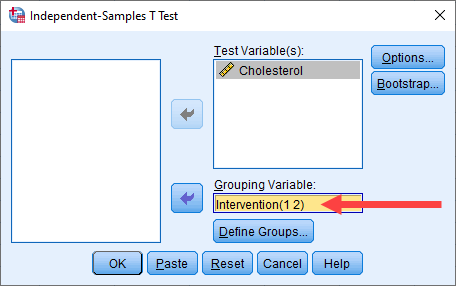
- Transfer the dependent variable, Cholesterol, into the Test Variable(s): box, by selecting it (by clicking on it) and then clicking on the top button. Next, transfer the independent variable, Intervention, into the Grouping Variable: box, by selecting it and then clicking on the bottom button. You will end up with the following screen:
Published with written permission from SPSS, IBM Corporation.
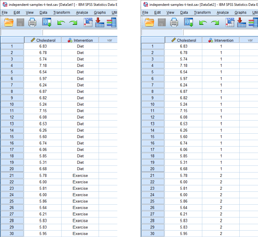
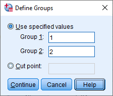
- Click on the button. You will be presented with the Define Groups dialogue box, as shown below:
Note: If the button is not active (i.e., it looks faded, like this ), click into the Grouping Variable: box to make sure that the independent variable (e.g., in our example, Intervention) is highlighted in yellow, as it is in Step 2 above. This will activate the button.
Published with written permission from SPSS, IBM Corporation.
- Enter "1" into the Group 1: box and "2" into the Group 2: box, as shown below:
Published with written permission from SPSS Statistics, IBM Corporation.
Explanation: You are entering "1" into the Group 1: box and "2" into the Group 2: box because this is how we coded the two groups of our categorical independent variable, Intervention, in the Value Labels dialogue box, as explained earlier and as shown below:
The Define Groups dialogue box is telling SPSS Statistics to carry out an independent-samples t-test using these two groups from our Value Labels dialogue box: 1 = "Diet" and 2 = "Exercise".
This may seem like an unnecessary step because our categorical independent variable clearly only has two groups (i.e., it is a dichotomous variable). However, we do it because your categorical independent variable could have more than two groups, but you simply decided to analyse only two groups. For example, imagine that our study collected data on cholesterol concentration amongst four groups: the two groups we have been discussing, "Diet" and "Exercise", but also "Drug" (where participants took a new cholesterol reducing drug for a 6-month period) and "Control" (where participants were not given any intervention). In this case, our Value Labels dialogue box would have the following four groups:
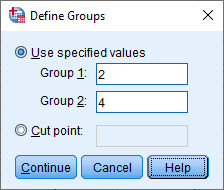
Therefore, two more groups have been added to the Value Labels dialogue box above: 3 = "Drug" and 4 = "Control". Now imagine that we only wanted to carrying out an independent-samples t-test to compare the differences in cholesterol concentration between the exercise group (i.e., 2 = "Exercise") and the control group (i.e., 4 = "Control"). In this case, we would enter "2" into the Group 1: box and "4" into the Group 2: box of the Define Groups dialogue box, as shown below:
- Click on the button. You will be returned to the Independent-Samples T Test dialogue box, but now with a completed Grouping Variable: box, as highlighted below:
Published with written permission from SPSS Statistics, IBM Corporation.
Explanation: In the previous step you entered "1" into the Group 1: box and "2" into the Group 2: box, which reflected the coding for our dichotomous independent variable, Intervention (i.e., "1 = Diet" and "2 = Exercise"). Therefore, after clicking on the button in the previous step, you should expect to see two pieces of information in the Grouping Variable: box: (a) the name of your independent variable (i.e., "Intervention" in our example); followed by (b), the coding of your two groups in brackets (i.e., "(1 2)" in our example). Therefore, the Grouping Variable: box above includes the text, "Intervention(1 2)".
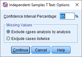
- Click on the button. You will be presented with the Independent-Samples T Test: Options dialogue box, as shown below:
Published with written permission from SPSS Statistics, IBM Corporation.
We use the Independent-Samples T Test: Options dialogue box to tell SPSS Statistics: (a) the alpha level (α) we want to set for our independent-samples t-test analysis, which affects the level at which you declare that a result is statistically significant (i.e., using a p-value under a NHST approach) and the confidence interval (CI) we use (i.e., under an estimation approach); and (b) how we want to deal with missing values in our data set when using an independent-samples t-test to analyse our data. The two options are briefly discussed below:
Note: If you are unfamiliar with the idea of p-values using a NHST approach or confidence intervals (CI) using an estimation approach, we introduced these concepts earlier in the section: Understanding why the independent-samples t-test is being used.
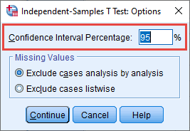
- The Confidence Interval Percentage box: Using a NHST approach, we set the level at which we declare that the independent-samples t-test result is statistically significant, which is known as the alpha level (α). By default in SPSS Statistics, the alpha level is set at .05 (i.e., α = .05), which is why the number "95" (i.e., 95%) is displayed in the Confidence Interval Percentage box, as highlighted below:
Published with written permission from SPSS Statistics, IBM Corporation.
Explanation: To explain the relationship between the alpha level (α) you set in your study and the number that is displayed in the Confidence Interval Percentage box, you start with the number "1" and subtract the alpha level (α). For example, 1 – (an alpha level of) .05 = .95 (i.e., 95%), so the number "95" is entered into the Confidence Interval Percentage box. If the alpha level (α) was 0.01, the number "99" would be entered into the Confidence Interval Percentage box (i.e., 1 - 0.01 = .99 or 99%).
An alpha level (α) of .05 means that if the statistical significance value (i.e., p-value) returned by SPSS Statistics when carrying out the independent-samples t-test is less than .05 (i.e., p < .05), we state that the mean difference in the dependent variable between the two groups of the independent variable is statistically significant. Therefore, we reject the null hypothesis that there is no mean difference between the two groups in the population and accept the alternative hypothesis that there is a mean difference between the two groups in the population. Alternatively, if the statistical significance value (i.e., p-value) is greater than .05 (i.e., p > .05), we state that the mean difference in the dependent variable between the two groups of the independent variable is not statistically significant. Therefore, we fail to reject the null hypothesis that there is no mean difference between the two groups in the population and reject the alternative hypothesis that there is a mean difference between the two groups in the population. It is important to note that you cannot accept the null hypothesis that there is no mean difference in the population.
The value you entered into the Confidence Interval Percentage box also determines the confidence interval (CI) that is set using an estimation approach. For example, by setting the level at 95% (i.e., the default in SPSS Statistics), this means that SPSS Statistics will produce a 95% confidence interval (CI) of the mean difference. Therefore, when you interpret the mean difference in the dependent variable between your two groups, SPSS Statistics will show the lower bound and the upper bound of this mean difference based on the 95% CI. For example, imagine that the mean difference in cholesterol concentration between the diet group and exercise group is 0.52 mmol/L. SPSS Statistics will also display the lower bound of the mean difference (e.g., 0.17 mmol/L) and the upper bound of the mean difference (e.g., 0.86 mmol/L) based on the 95% CI, which indicates a plausible range of values that the mean difference could be in the population.
If you want to change the alpha level (α) and the 95% CI, you simply enter the value you want to use between 1 and 99 in the Confidence Interval Percentage box. For example, if you changed the value to "99" in the Confidence Interval Percentage box, a 99% CI would be applied when carrying out your independent-samples t-test analysis, which would also mean declaring statistical significance at the p < .01 level (i.e., declaring statistical significance when the p-value returned by SPSS Statistics is less than .01).
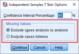
- The –Missing Values– area: When we entered the data for our example into the Data View window of SPSS Statistics, as explained in the Data Setup section earlier, we entered 40 values for the dependent variable, Cholesterol, under the column, which represented the 40 participants in our study: 20 participants in the exercise group and 20 participants in the diet group. If we had not entered a value under the column for all 40 participants, we would have missing data.
When carrying out an independent-samples t-test, SPSS Statistics provides two options when you have missing data, which are Exclude cases analysis by analysis and Exclude cases listwise, as highlighted in the –Missing Values– area below:
Published with written permission from SPSS Statistics, IBM Corporation.
If you do not having missing data, you can ignore the –Missing Values– area. If you have missing data and you are only carrying out one independent-samples t-test, you can also ignore the –Missing Values– area because the results that are produced by SPSS Statistics will be the same when selecting Exclude cases analysis by analysis or Exclude cases listwise. Therefore, in our example, we do not need to make any changes in the –Missing Values– area.
Alternatively, if you have missing data and have more than one dependent variable that you are investigating, you need to consider the Exclude cases analysis by analysis and Exclude cases listwise options because they will affect how SPSS Statistics deals with missing values in your data set when carrying out an independent-samples t-test. If this is of interest, we explain how selecting these two different options will affect your results in our enhanced independent-samples t-test guide, which you can access by subscribing to Laerd Statistics.
Therefore, in our example we have not made any changes to the options in the Independent-Samples T Test: Options dialogue box. Instead, we are using the default settings because: (a) we want to test the statistical significance of the mean difference between our two groups using an alpha level (α) of .05; (b) we want SPSS Statistics to report the 95% CI of the mean difference; and (c) we are carrying out only one independent-samples t-test (and have no missing data).
- Click on the button. You will be returned to the Independent-Samples T Test dialogue box.
- Click on the button to generate the results of your independent-samples t-test analysis.
The results from the independent-samples t-test analysis above are discussed in the next section: Interpreting the results of an independent-samples t-test analysis.
SPSS Statistics
Interpreting the results of an independent-samples t-test analysis
After carrying out an independent-samples t-test in the previous section, SPSS Statistics displays the results in the IBM SPSS Statistics Viewer using two tables: the Group Statistics table and the Independent Samples Test table.
If your data "passed/met" assumption #4 (i.e., you do not have problematic outliers), assumption #5 (i.e., your dependent variable is normally distributed for each category of your independent variable) and assumption #6 (i.e., you have homogeneity of variances), you only need to interpret the results in these two tables. Furthermore, you still only have to interpret these two tables if your data "violated/did not meet" assumption #6 (i.e., you do not have homogeneity of variances, which means that you have heterogeneity of variances). However, if your data "violated/did not meet" assumption #4 and/or assumption #5, the results in the Independent Samples Test table might be invalid/inaccurate and it is possible that the conclusions you make about your results would also be incorrect. Instead, you will have to make changes to your data and/or run a different statistical test to analyse your data. We explain how to test whether your data "passes/meets" these assumptions in our enhanced independent-samples t-test guide, which you can access by subscribing to Laerd Statistics. We also explain what options you have when these assumptions are "violated/not met", as well as providing guides to help you continue with your analysis. However, in this introductory guide to the independent-samples t-test, we explain how to interpret your results when your data "passed/met" assumptions #4, #5 and #6. We do this over the four sections that follow: (1) understanding descriptive statistics; (2) the independent-samples t-test results using an "estimation" approach (using 95% CI); (3) the independent-samples t-test results using a "Null Hypothesis Significance Testing" (NHST) approach (using p-values); and (4) effect size calculations after carrying out an independent-samples t-test.
Understanding descriptive statistics when interpreting your independent-samples t-test results
When interpreting the results from an independent-samples t-test, descriptive statistics help you get a "feel" for your data, as well as being used when reporting the results of your independent-samples t-test analysis. Such descriptive statistics include the sample size, sample mean and sample standard deviation for each group of your independent variable, as well as the sample mean difference between these two groups.
The sample size, sample mean and sample standard deviation are shown in the Group Statistics table, whilst the sample mean difference is shown in the Independent Samples Test table. In this section, we discuss each of these tables in turn, starting with the Group Statistics table below:
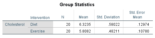
Published with written permission from SPSS Statistics, IBM Corporation.
The Group Statistics table has two rows – one row for each group of the independent variable – with the columns presenting descriptive statistics for each group. In our example, the descriptive statistics for the "Diet" group are displayed on the first row, whilst the descriptive statistics for the "Exercise" group are displayed on the second row. These descriptive statistics have the following meaning:
| |
Column Name |
Meaning |
| 1 |
N |
The number of cases (i.e., the number of participants in our example) for each group of the independent variable (i.e., for the "Diet" and "Exercise" groups of the independent variable, Intervention, in our example). |
| 2 | Mean |
The sample mean (i.e., the "average" score) for each group of the independent variable, which is the measure of central tendency used in an independent-samples t-test.
If your data "violated/did not meet" assumption #4 and/or assumption #5, the mean may not be an appropriate measure of central tendency and you may need to use a different measure of central tendency (e.g., a trimmed mean). |
| 3 | Std. Deviation |
The sample standard deviation for each group of the independent variable, which is the measure of spread "typically" used in an independent-samples t-test. |
| 4 |
Std. Error Mean |
The standard error of the mean for each group of the independent variable. |
| Table 1: Explanation of the Group Statistics table. |
In summary, the Group Statistics table presents the sample size (i.e., under the "N" column), the sample mean (i.e., under the "Mean" column), the sample standard deviation (i.e., under the "Std. Deviation" column), and the standard error of the mean (i.e., under the "Std. Error Mean" column), for the diet group and exercise group (i.e., along rows "Diet" and "Exercise" rows respectively).
You should use the Group Statistics table to understand: (a) whether there are an equal number of participants in each of your groups (i.e., under the "N" column): (b) which group had the higher/lower mean score (i.e., under the "Mean" column), and what this means for your results; and (c) if the variation of scores in each group is similar (e.g., under the "Std. Deviation" column).
Whilst both the standard deviation and standard error of the mean are used to describe data, the standard error of the mean is considered to be erroneous in many of the cases where it is presented (e.g., see the discussion by Carter (2013) and explanation by Altman & Bland (2005)). Therefore, you would typically report the sample mean and sample standard deviation (and not the standard error of the mean).
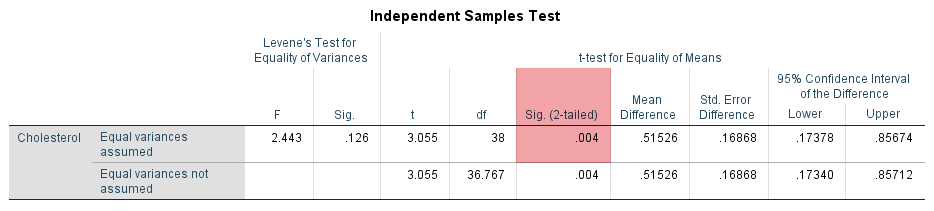
The results show that the mean cholesterol concentration in the diet group was 6.32 mmol/L (to 2 decimal places) with a standard deviation of 0.58 mmol/L (again reported to 2 decimal places). There were 20 participants in the diet group. In the exercise group, mean cholesterol concentration was 5.81 mmol/L with a standard deviation of 0.48 mmol/L. There were also 20 participants in the exercise group. Therefore, there was a mean difference of 0.52 mmol/L (to 2 decimal places) between the diet group and exercise group in our two samples, with cholesterol concentration being 0.52 mmol/L higher in the diet group (i.e., 6.3235 – 5.8082 = 0.52 mmol/L to 2 decimal places). This sample mean difference is also show in the Independent Samples Test table, as highlighted below:
Published with written permission from SPSS Statistics, IBM Corporation.
The descriptive statistics in this section help us to understand our sample data, highlighting the mean cholesterol concentration, standard deviation and the mean difference between our two groups. In other words, we now know the sample mean, sample standard deviation and sample mean difference. However, we are not only interested in our sample, but the population from which the sample was drawn, as discussed earlier in the section: Understanding why the independent-samples t-test is being used. Therefore, in the next two sections we focus on the mean difference in the population (i.e., the population mean difference), first using an estimation approach (using 95% CI) and then using a NHST approach (using p-values).
Understanding the independent-samples t-test results under an "estimation" approach (using a 95% CI)
So far, we know that the mean difference in cholesterol concentration between the diet group and exercise group in our two samples is 0.52 mmol/L (to 2 decimal places). However, we also know from our discussion earlier that this sample mean difference of 0.52 mmol/L is based on only a single study of one sample of 20 participants in the diet group and another sample of 20 participants in the exercise group, and not from the millions of sedentary people that this study could theoretically represent. If we carried out a second study with a sample of 20 participants in the diet group and a sample of 20 participants in the exercise group, or a third study with a sample of 20 participants in the diet group and a sample of 20 participants in the exercise group, or a fourth study with a sample of 20 participants in the diet group and a sample of 20 participants in the exercise group, it is likely that the mean difference in cholesterol concentration will be different each time, or at least, most of the time (e.g., 0.18 mmol/L in the second study, 0.92 mmol/L in the third study, 0.57 mmol/L in the fourth study). In other words, there will be some variation in the sample mean difference each time we sample our populations.
Since we have just one study and we know that there will be some variation in the mean difference and standard deviation in cholesterol concentration between participants in the diet group and exercise group each time we sample our population, we need a way to assess the uncertainty in estimating the population mean difference based on our sample mean difference of 0.52 mmol/L (i.e., there is some error in the sample mean difference that is being used to estimate the population mean difference). Therefore, we use an independent-samples t-test to help us quantify this error (i.e., the error between the mean difference in our sample when compared to the mean difference in our population).
As previously stated, the sample mean difference is the best estimate of the population mean difference, but since we have just one study where we took a single sample from each of our two populations, we know that this estimate of the population mean difference in cholesterol concentration between participants in the diet group and exercise group will vary (i.e., it will not always be the same as in this study). In order to quantify this uncertainty in our estimate of the population mean difference, we can use the independent-samples t-test to provide a 95% confidence interval (CI), which is a way of providing a measure of this uncertainty. Presenting a mean difference with a 95% CI to understand what the population mean difference is, and your uncertainty in its value, is an approach called "estimation".
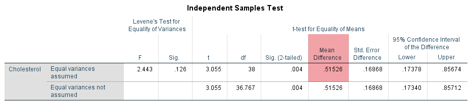
One approach to quantify the uncertainty in using the sample mean difference to estimate the population mean difference is to use a confidence interval (CI). When doing so, you can set different levels of confidence for your confidence interval (CI). As discussed earlier in the Procedure section, the most common confidence interval (CI) is the 95% CI, which is the default in SPSS Statistics (and most statistics packages), and is what is reported under the "95% Confidence Interval of the Difference" column in the Independent Samples Test table, as highlighted in orange below:
Published with written permission from SPSS Statistics, IBM Corporation.
A confidence interval (CI) will give you, based on your sample data, a likely/plausible range of values that the mean difference might be in the population. For example, we know that the mean difference in cholesterol concentration between participants in the diet group and exercise group in our two samples was 0.52 mmol/L, as highlighted in the "Mean Difference" column in the table above. Furthermore, we know from the Group Statistics table earlier that cholesterol concentration was 0.52 mmol/L higher in the diet group (i.e., 6.3235 – 5.8082 = 0.52 mmol/L to 2 decimal places).
A 95% CI, which is reported under the "95% Confidence Interval of the Difference" column in the Independent Samples Test table above, could suggest that the mean difference in cholesterol concentration between people who undertake a 6-month dietary programme (i.e., the diet group) and people who undertake a 6-month exercise programme (i.e., the exercise group) in the population might plausibly be somewhere between 0.17 mmol/L and 0.86 mmol/L (both to 2 decimal places). Here, 0.17 mmol/L reflects the lower bound of the 95% CI, reported under the "Lower" column, and 0.86 mmol/L reflects the upper bound of the 95% CI, reported under the "Upper" column.
The 95% CI is a very useful method to quantify the uncertainty in using the sample mean difference to estimate the population mean difference because although the sample mean difference is the best estimate that you have of the population mean difference, in reality, the mean difference in the population could plausibly be any value between the lower bound and upper bound of the 95% CI. If you choose to increase the CI when carrying out an independent-samples t-test from, for example, 95% to 99%, you increase your level of confidence that the population mean difference is somewhere between the lower and upper bounds that are reported.
Therefore, based on our two samples of 20 participants in the diet group and 20 participants in the exercise group, it appears that sedentary people in the population who undertake a 6-month exercise programme may have lower cholesterol concentration at the end of such a programme compared to sedentary people who undertake a 6-month dietary programme. The results from the independent-samples t-test analysis suggest that cholesterol concentration could plausibly be somewhere between 0.17 mmol/L and 0.86 mmol/L lower amongst sedentary people who undertake a 6-month exercise programme compared to sedentary people who undertake a 6-month dietary programme.
In the section, Calculating an effect size based on your independent-samples t-test results, we highlight the need to discuss the practical significance of this result; in other words, the need to discuss whether from a health perspective, a mean difference in cholesterol concentration that could plausibly be between 0.17 mmol/L and 0.86 mmol/L amongst sedentary people in the population who undertake a 6-month exercise programme compared to a 6-month dietary programme may be important or at least interesting. However, in the next section we first discuss how to interpret the independent-samples t-test results using a Null Hypothesis Significance testing (NHST) approaching using p-values.
Understanding the independent-samples t-test results under a "Null Hypothesis Significance Testing" (NHST) approach (using p-values)
As we discussed in the previous section, we know that the mean difference in cholesterol concentration between the diet group and exercise group in our two samples is 0.52 mmol/L (to 2 decimal places). We also know that this sample mean difference of 0.52 mmol/L is based on just a single study of one sample of 20 participants in the diet group and another sample of 20 participants in the exercise group, and not from the millions of sedentary people that this study could theoretically represent. Knowing this information, sometimes the main goal of a study is simply to answer the question: Is there a mean difference between your two groups in the population? This is the goal of Null Hypothesis Significance Testing (NHST).
Note: As we mentioned earlier, unless you are familiar with statistics, the idea of NHST can be a little challenging at first and benefits from a detailed description, but we will try to give a brief overview in this section. However, since it can be challenging to understand how the independent-samples t-test is used under NHST, we will be adding a guide dedicated to explaining this, including concepts such as the t-distribution, alpha (ɑ) levels, statistical power, Type I and Type II errors, p-values, and more. If you would like us to let you know when we add this guide to the site, please contact us.
Using NHST, the independent-samples t-test is used to test the null hypothesis that there is no mean difference between your two groups in the population, based on the data from your single study. For example, it tests that null hypothesis that there is no mean difference in cholesterol concentration between participants in the diet group and exercise group in the population. Furthermore, the independent-samples t-test is typically used to test the null hypothesis that the mean difference between the two groups in the population is zero (e.g. a mean difference of 0 mmol/L in cholesterol concentration between participants in the diet group and exercise group), which is also referred to as the nil hypothesis, but it can be tested against a specific value (e.g., a mean difference of 0.85 mmol/L in cholesterol concentration between participants in the diet group and exercise group). Whilst the null hypothesis states that there is no mean difference between your two groups in the population, the alternative hypothesis states that there is a difference between your two groups in the population (e.g., the alternative hypothesis that the mean difference in cholesterol concentration between participants in the diet group and exercise group is not 0 mmol/L or the specific value you set, such as 0.85 mmol/L, in the population).
The p-value calculated as part of NHST is the probability of finding a result as extreme or more extreme than the result in your study, given that the null hypothesis is true. If your result – or one more extreme – is unlikely to have happened by chance (i.e., due to sampling variation), you make the declaration that you believe the null hypothesis is false (i.e., there is a mean difference between the two groups in the population). NHST does not say what this difference might be.
Determining whether to reject or fail to reject the null hypothesis is based on a preset probability level (i.e., sometimes called an alpha (ɑ) level). This alpha (ɑ) level is usually set at .05, which means that if the p-value is less than .05 (i.e., p < .05), you declare the result to be statistically significant, such that you reject the null hypothesis and accept the alternative hypothesis. Alternatively, if the p-value is greater than .05 (i.e., p > .05), you declare the result to be not statistically significant, such that you fail to reject the null hypothesis and reject the alternative hypothesis.
These concepts can be fairly difficult to understand without further explanation, but for the purpose of this introductory guide, the important point is that the independent-samples t-test will produce a p-value that can be used to either (a) reject the null hypothesis of no mean difference in the population and accept the alternative hypothesis that there is a mean difference; or (b) fail to reject the null hypothesis, suggesting that there is not enough evidence to accept the alternative hypothesis that there is a mean difference in the population (i.e., rejecting the alternative hypothesis that there is a mean difference). It is important to note that you cannot accept the null hypothesis that there is no mean difference.
The p-value for the independent-samples t-test can be found under the "Sig. (2-tailed)" column of the Independent Samples Test table, as highlighted below:
Published with written permission from SPSS Statistics, IBM Corporation.
The p-value reported under the "Sig. (2-tailed)" column above is used to determine if there is a statistically significant mean difference between your two groups. If p < .05 (i.e., if p is less than .05), there is a statistically significant mean difference in cholesterol concentration between the diet group and exercise group. If p > .05 (i.e., if p is greater than .05), there is not a statistically significant mean difference in cholesterol concentration between the diet group and exercise group. Since p = .004 in our example, there is a statistically significant mean difference in cholesterol concentration between the diet group and exercise group. In other words, the results suggest that there is a mean difference in the population based on the sample that was studied.
Based on this result, we can reject the null hypothesis of no mean difference in the population and accept the alternative hypothesis that there is a mean difference. Notice that we use words like "suggest" when describing our results. This is important because we are using the independent-samples t-test to assess whether our sample data gives us reason to believe that we should accept the alternative hypothesis at a certain level of probability. In our example, this level of probability is set at the alpha level (α) of .05, which is why we assess whether our result is statistically significant (or not) based on a p-value that is less than or greater than .05 respectively.
Note: The independent-samples t-test is based on the t distribution, so when assessing the results from an independent-samples t-test, the obtained t-value and degrees of freedom (df) of the test should be reported. These can be found in the "t" and "df" columns of the Independent Samples Test table below:
In the Independent Samples Test table above, the obtained t-value is 3.06 (to 2 decimal places), reported under the "t" column, and the degrees of freedom (df) are 38, reported under the "df" column (i.e., for an independent-samples t-test with equal variances, the degrees of freedom are equal to the sample size minus 2, so in our example, 40 – 2 = 38).
A major criticism of NHST is that it results in a dichotomous decision where you simply conclude that there either is a mean difference between your two groups in the population or there is not a mean difference. Therefore, it provides far less information that the 95% CI discussed in the previous section, which is now the preferred approach. Nonetheless, when carrying out an independent-samples t-test, it is common to interpret and report both the p-value and 95% CI.
In the next section, Calculating an effect size based on your independent-samples t-test results, we highlight the need to discuss the practical significance of our results.
Calculating an effect size based on your independent-samples t-test results
As explain in the earlier section, Understanding why the independent-samples t-test is being used, the independent-samples t-test: (a) using the NHST approach, gives you an idea of whether there is a mean difference between your two groups in the population, based on your sample data; and (b) as a method of estimation using confidence intervals (CI), provides a plausible range of values that the mean difference between your two groups could be in the population, based on your sample data. However, the NHST approach does not indicate the "size" of the mean difference, unlike the estimation approach. Also, neither approach provide a standardised effect size.
As an introduction to effect size measures, these can be classified into two categories: unstandardised and standardised.
- Unstandardized effect sizes: An unstandardised effect size is reported using the units of measurement of the dependent variable. In our example, the dependent variable, cholesterol concentration, is being measured using mmol/L. Therefore, imagine that the mean difference in cholesterol concentration between the exercise group and diet group after the 6-month intervention is 0.52 mmol/L. The unstandardised effect size would be 0.52 mmol/L. To take another example we used earlier in this guide, if the mean difference in weekly screen time between male and female university students was 27 minutes, then 27 minutes is the unstandardised effect size (i.e., the dependent variable, weekly screen time, was measured in minutes).
- Standardized effect sizes: A standardised effect size removes the units of measurement (i.e., they are unitless) due to the standardisation. Therefore, standardised effect sizes are useful when: (a) the units of measurement of the dependent variable are not meaningful/intuitive (e.g., a dependent variable such as job satisfaction, which may be created by totalling or averaging the scores from multiple 5-point Likert item questions in a survey); and/or (b) when you want to compare the "size" of an effect between different studies (e.g., the effect of an exercise and dietary intervention on cholesterol concentration reported in different studies).
In our example, we would first report the unstandardised effect size, which is 0.52 mmol/L. After all, to any health practitioner who deals with cholesterol levels in patients, a mean difference of 0.52 mmol/L in cholesterol concentration amongst sedentary people suggests that the findings from this (fictitious) study "might be" of practical importance. In other words, the mean difference in this "amount" of cholesterol concentration suggests that the effect of a 6-month exercise programme compared to 6-month dietary programme is worthy of further research. If further research consistently suggests that an exercise programme leads to lower cholesterol concentrations in participants compared to a dietary programme by an "average" of around 0.52 mmol/L, this may influence the advice health practitioners give patients, as well as influencing what type of programmes the Government invests in to reduce cholesterol concentration amongst sedentary people.
However, it is important to also take into account the 95% CI that were produced as part of our analysis. After all, the 95% CI suggested that the mean difference in cholesterol concentration between the exercise group and diet group in the population may plausibly be anywhere between 0.17 mmol/L and 0.86 mmol/L (i.e., any value between the "lower bound" and "upper bound" of the 95% CI). Therefore, a health practitioner analysing the results from this single study would have to ask the question: If the unstandardised effect size was only 0.17 mmol/L (i.e., the "lower bound" of the 95% CI), would the results from this study still be of practical importance? In other words, if the effect of a 6-month exercise programme compared to 6-month dietary programme is only a reduction in cholesterol concentration of 0.17 mmol/L, would these results still influence the decisions make by health practitioners or influence health policy more broadly (i.e., would the results still influence whether health practitioners recommended a 6-month exercise programme rather than a dietary programme to help sedentary people reduce their cholesterol concentration)?
After reporting the unstandardised effect size, we might also report a standardised effect size such as Cohen's d (Cohen, 1988). In our example, this may be useful for future studies where researchers want to compare the "size" of the effect in their studies to the size of the effect in this study.
There are many different types of standardised effect size, with different types often trying to "capture" the importance of your results in different ways. Unfortunately, SPSS Statistics does not automatically produce an effect size as part of an independent-samples t-test analysis. However, it is easy to calculate a standardised effect size such as Cohen's d using the results from the independent-samples t-test analysis. Therefore, we show you how to calculate and interpret Cohen's d in our enhanced independent-samples t-test guide, which you can access by subscribing to Laerd Statistics.
In the next section of this introductory guide, we explain how to report the results of an independent-samples t-test.
SPSS Statistics
Reporting the results from an independent-samples t-test analysis
When you report the results of an independent-samples t-test, it is good practice to include the following information:
- A. An introduction to the analysis you carried out, which includes: (a) the statistical test being used to analyse your data (i.e., the independent-samples t-test); (b) the continuous dependent variable being measured (e.g., cholesterol concentration, in our example); and (c) the two groups of the independent variable that are being compared (e.g., sedentary participants in our example), in line with Assumptions #1 and #2.
- B. Information about your sample, including the number of participants (n) in each of your two groups. This is useful to understand whether you have a balanced or unbalanced design (i.e., whether there were an equal or unequal number of participants between the two groups), as well as highlighting any missing values.
- C. A statement to indicate how you helped to ensure independence of observations, as discussed in Assumption #3.
- D(i). If the independent-samples t-test is being used under a NHST approach, a statement of whether there was a statistically significant mean difference between your two groups, including the group means (Mean), standard deviations (Std. Deviation), estimated mean difference (Mean Difference), t-value (t), degrees of freedom (df) (df), and statistical significance value (i.e., the p-value) (Sig. (2-tailed)).
You can also include a statement of whether the statistical significance value (i.e., the p-value) calculated by the independent-samples t-test leads you to: (a) reject the null hypothesis of no mean difference in the population and accept the alternative hypothesis that there is a mean difference; or (b) fail to reject the null hypothesis, suggesting that there is not enough evidence to accept the alternative hypothesis that there is a mean difference in the population (i.e., rejecting the alternative hypothesis that there is a mean difference). It is important to note that you cannot accept the null hypothesis that there is no mean difference.
- D(ii). If the independent-samples t-test is being used under an estimation approach, a statement of whether there was a mean difference between your two groups, including the group means (Mean), standard deviations (Std. Deviation), estimated mean difference (Mean Difference), 95% confidence interval (CI) for the mean difference (95% Confidence Interval of the Difference), t-value (t), degrees of freedom (df) (df), and statistical significance value (i.e., the p-value) (Sig. (2-tailed)). Note that you are reporting both the p-value and 95% CI, is now the preferred approach.
- E. A measure of effect size, which is a method of demonstrating the practical/clinical importance of your results. In an independent-samples t-test, the effect size demonstrates the practical/clinical importance of the mean difference between your two groups. You can report the unstandardised effect size, or both the unstandardised effect size and a standardised effect size (e.g., a standardised effect size such as Cohen's d).
- F. A table of your results if you have conducted two or more independent-samples t-tests. Whilst a table can be used when you have only carried out one independent-samples t-test, as in our example, it often makes sense to simply report such results in-text rather than using a table. In contrast, tables are useful when you have a lot more results to report (i.e., when you have carried out multiple independent-samples t-tests).
- G. A suitable graph to illustrate the means and distribution/spread of scores of your two groups (e.g., the distribution/spread of cholesterol concentration scores for the exercise group and diet group in our example). The choice of graph can depend on personal preferences, but also the size of your sample.
Note: Whilst you can present your results in-text, using a table and a graph, many reporting styles do not favour the duplication of results using all three methods. For example, if your results are explained in detail in-text, the use of a table and/or graph may be viewed as an unnecessary duplication. However, if you do not have to work to a specific reporting style, simply make sure that you are fully explaining your results in a way that the reader can understand, irrespective of whether you do this in-text, using a table and/or a graph.
Based on the results from the independent-samples t-test and associated descriptive statistics in the previous section, we could report the results of this fictitious study using an estimation approach as follows:
An independent-samples t-test was run on a random sample of 40 sedentary individuals to determine if there was a mean difference in cholesterol concentration between participants who underwent a 6-month exercise intervention and a 6-month dietary intervention. There were 20 participants in the exercise intervention group and 20 in the dietary intervention group, who were randomly assigned to each group. At the end of the 6-month study, the results showed that cholesterol concentration was lower in the exercise group (5.81 ± 0.48 mmol/L) compared to the diet group (6.32 ± 0.58 mmol/L), a mean difference of 0.52 (95% CI, 0.17 to 0.86) mmol/L, t(38) = 3.06, p = .004.
The results from an independent-samples t-test can be illustrated using different types of graph, depending on what you are trying to highlight and the characteristics of your data (e.g., the size of your sample). One such graph is a jittered dot plot with superimposed mean and standard deviation "error bars", as highlighted below:
A jittered dot plot with superimposed mean and standard deviation "error bars" shows:
- A. The values for the dependent variable on the y-axis for the two groups displayed on the x-axis. Therefore, in our example, cholesterol concentration is displayed on the y-axis, measured in mmol/L, and the two groups of our independent variable, the "Diet" group and the "Exercise" group are displayed on the x-axis.
- B. The mean score for each group of the independent variable as a bold black dot in the middle of the dot plot.
- C. The individual scores along the y-axis for each group of the independent variable, where each lighter coloured black/grey dot represents a single case (e.g., participant) in your data set.
- D. The standard deviation "error bars" (i.e., one above and one below the mean score) for each group of the independent variable, which give you an idea of the variability (i.e., spread) of the scores.
The information from this jittered dot plot helps to highlight that:
- A. The mean cholesterol concentration was higher in the "Diet" group who undertook a 6-month dietary programme compared to the "Exercise" group who undertook a 6-month exercise programme.
- B. The distribution of cholesterol concentration scores was more clustered around the mean in the "Exercise" group compared to the "Diet" group (i.e., there was less variation in the cholesterol concentration scores amongst participants in the exercise group).
The jittered dot plot is also useful when discussing outliers, which is an important assumption of the independent-samples t-test. However, it should be stressed that the jittered dot plot alone would be insufficient to test whether your data has met this assumption.
Note: This completes our introductory guide to the independent-samples t-test using SPSS Statistics. In our enhanced independent-samples t-test guide, we show you how to write up the results from your assumptions tests and independent t-test procedure if you need to report this in a dissertation/thesis, assignment or research report. We do this using the Harvard and APA styles. You can access our enhanced independent-samples t-test guide by subscribing to Laerd Statistics. However, if you have any comments/feedback about this guide or if you would like us to add other guides to Laerd Statistics, please contact us and let us know how we can help.
SPSS Statistics
Bibliography and Referencing
Please see the list below:
| Book |
Altman, D. G. (1999). Practical statistics for medical research. London: Chapman & Hall. |
| Journal Article |
Altman, D. G., & Bland, J. M. (2005). Standard deviations and standard errors. BMJ, 331(7521), 903. |
| Journal Article |
Barde, M. P, & Barde, P. J. (2012). What to use to express the variability of data: Standard deviation or standard error of mean? Perspect Clin Res, 3, 113-6. |
| Journal Article |
Carter, R. E. (2013). A standard error: Distinguishing standard deviation from standard error. Diabetes, 62, e15. |
| Book |
Cohen, J. (1988). Statistical power analysis for the behavioral sciences (2nd ed.). Hillsdale, NJ: Lawrence Erlbaum Associates. |
| Book |
Fowler, J., & Cohen, L. (1990). Practical statistics for field biology. West Sussex, UK: Open University Press. |
| Book |
Fox, J. (2008). Applied regression analysis and generalized linear models (2nd ed.). Thousand Oaks, CA: Sage Publications. |
| Book |
Fox, J. (2016). Applied regression analysis and generalized linear models (3rd ed.). Thousand Oaks, CA: Sage Publications. |
| Journal Article |
Glantz, S. A. (1980). Biostatistics: How to detect, correct and prevent errors in the medical literature. Circulation, 61, 1-7. |
| Book |
Howell, D. C. (2010). Statistical methods for psychology (7th ed.). Belmont, CA: Wadsworth. |
| Book |
Judd, C. M., McClelland, G. H., & Ryan, C. S. (2009). Data analysis: A model comparison approach (2nd ed.). New York: Routledge. |
| Conference Paper |
Kang, Y., & Harring, J. R. (2012). Investigating the impact of non-normality, effect size, and sample size on two-group comparison procedures: An empirical study. Presented at the annual meeting of the American Educational Research Association (AERA), SIG: Educational Statisticians, Vancouver, BC. |
| Book |
Myers, J. L., Well, A. D., & Lorch, R. F., Jr. (2010). Research design and statistical analysis (3rd ed.). New York: Routledge. |
| Journal Article |
Nagale, P. (2003). Misuse of standard error of the mean (SEM) when reporting variability of a sample. A critical evaluation of four anaesthesia journals. BJA, 90(4), 514-516. |
| Book |
Osborne, J. W., & Overbay, A. (2008). Best practices in data cleaning: How outliers and "fringeliers" can increase error rates and decrease the quality and precision of your results. In J. W. Osborne (Ed.), Best practices in quantitative methods (pp. 205-213). Thousand Oaks, CA: Sage Publications. |
| Book |
Pedhazur, E. J. (1997). Multiple regression in behavioral research (3rd ed.). Fort Worth, TX: Wadsworth/Thomson Learning. |
| Book |
Piegorsch, W. W., & Bailer, A. J. (1997). Statistics for environmental biology and toxicology. London: Chapman & Hall. |
| Journal Article |
Satterthwaite, F. E. (1946). An approximate distribution of estimates of variance components. Biometrics Bulletin, 2, 110-114. |
| Book |
Sheskin, D. J. (2011). Handbook of parametric and nonparametric statistical procedures (5th ed.). Boca Raton, FL: Chapman & Hall/CRC Press. |
| Journal Article |
Welch, B. L. (1947). The generalization of "Student's" problem when several different population variances are involved. Biometrika, 34(1–2), 28–35. |
| Book |
Wilcox, R. (2012). Modern statistics for the social and behavioral sciences: A practical introduction. Boca Raton, FL: CRC Press. |
| Journal Article |
Zaugg, C. E. (2003). Standard error as standard. Circulation, 107, e89. |
SPSS Statistics
Reference this article
Laerd Statistics (2019). Independent-samples t-test using SPSS Statistics. Statistical tutorials and software guides. Retrieved Month, Day, Year, from https://statistics.laerd.com/spss-tutorials/independent-t-test-using-spss-statistics.php
For example, if you viewed this guide on 12th January 2020, you would use the following reference:
Laerd Statistics (2019). Independent-samples t-test using SPSS Statistics. Statistical tutorials and software guides. Retrieved January, 12, 2020, from https://statistics.laerd.com/spss-tutorials/independent-t-test-using-spss-statistics.php