Login

ANOVA with Repeated Measures using SPSS Statistics (cont...)

SPSS Statistics version 24
and earlier versions of SPSS Statistics
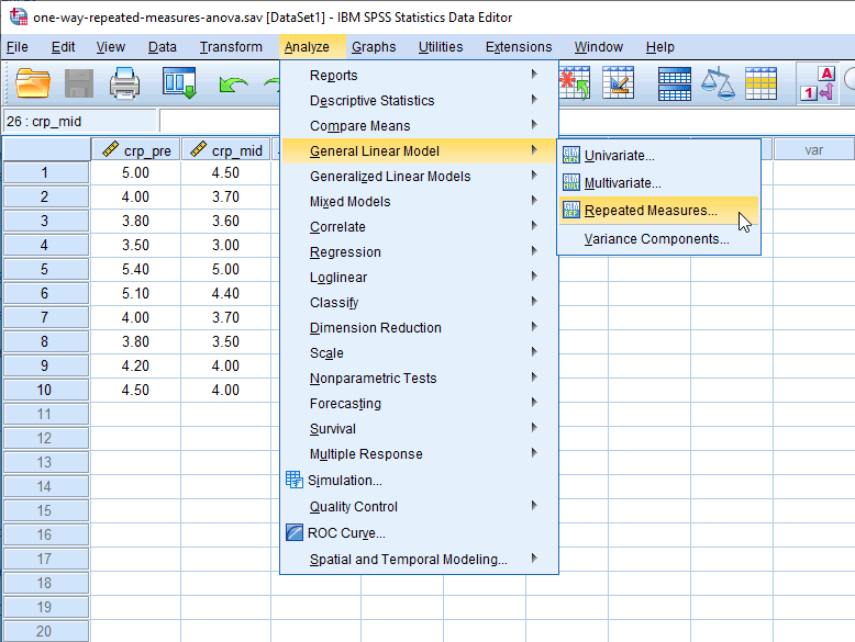
  1. Click Analyze > General Linear Model > Repeated measures... on the top menu, as shown below:
    Menu for the one-way repeated measures ANOVA in SPSS Statistics

    Published with written permission from SPSS Statistics, IBM Corporation.


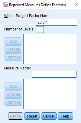
    You will be presented with the Repeated Measures Define Factor(s) dialogue box, as shown below:
    'Repeated Measures Define Factor(s)' dialogue box. Repeated measures ANOVA in SPSS. 'Within-Subject Factor Name' box at top

    Published with written permission from SPSS Statistics, IBM Corporation.

    Explanation: This dialogue box is where you inform SPSS Statistics that the three variables – crp_pre, crp_mid and crp_post – are three levels of the within-subjects factor, time. Without doing this, SPSS Statistics will think that the three variables are just that, three separate variables.

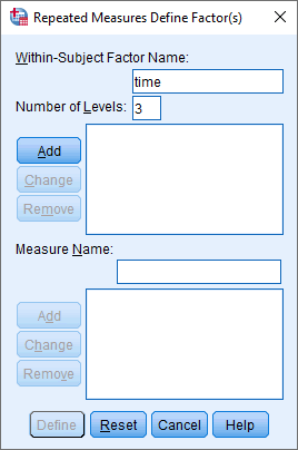
  2. In the Within-Subject Factor Name: box, replace "factor1" with a more meaningful name for your within-subjects factor. For example, we replaced "factor1" with "time" because this is the name of our within-subjects factor (i.e., time). Next, enter the number of levels of your within-subjects factor into the Number of Levels: box. For example, our within-subjects factor, time, has three levels, representing the three time points when our dependent variable, CRP, was measured (i.e., pre-intervention, crp_pre, mid-intervention, crp_mid, and post-intervention, crp_post). Therefore, we entered "3" into the Number of Levels: box, as shown below:
    'Repeated Measures Define Factor(s)' dialogue box. One-way repeated measures ANOVA in SPSS. 'time(3)' entered

    Published with written permission from SPSS Statistics, IBM Corporation.


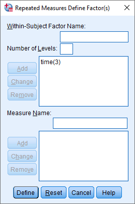
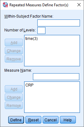
    Click on the Add button and you will be presented with the following screen:
    'Repeated Measures Define Factor(s)' dialogue box. One-way repeated measures ANOVA in SPSS. 'time(3)' added

    Published with written permission from SPSS Statistics, IBM Corporation.

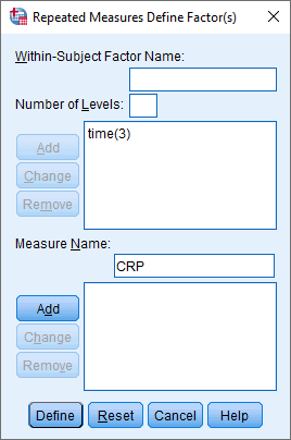
  3. In the Measure Name: box, enter a name that reflects the name of your dependent variable. Since our dependent variable is CRP, we entered "CRP", as shown below:
    'Repeated Measures Define Factor(s)' dialogue box. One-way repeated measures ANOVA in SPSS. 'CRP' entered

    Published with written permission from SPSS Statistics, IBM Corporation.


    Click on the Add button and you will get the following screen:
    'Repeated Measures Define Factor(s)' dialogue box. One-way repeated measures ANOVA in SPSS. 'CRP' added

    Published with written permission from SPSS Statistics, IBM Corporation.

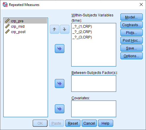
  4. Click on the Define button and you will be presented with the Repeated Measures dialogue box, as shown below:
    'Repeated Measures' dialogue box. Repeated measures ANOVA SPSS. Variables 'pre', 'mid' & 'post' on left

    Published with written permission from SPSS Statistics, IBM Corporation.

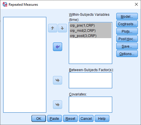
  5. Transfer crp_pre, crp_mid and crp_post into the "_?_(1,CRP)", "_?_(2,CRP)" and "_?_(3,CRP)" placeholders respectively in the Within-Subjects Variables (time): box, by highlighting all the variables in the left-hand box (by clicking on them whilst holding down the shift-key), and then clicking on the top right arrow button. You will end up with the following screen:
    'Repeated Measures' dialogue box Repeated measures ANOVA SPSS. Variables transferred to 'Within-Subjects Variables(time)' box

    Published with written permission from SPSS Statistics, IBM Corporation.

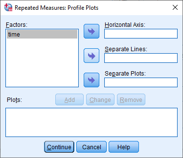
  6. Click on the Plots button. You will be presented with the Repeated Measures: Profile Plots dialogue box, as shown below:
    'Repeated Measures: Profile Plots' dialogue box. One-way repeated measures ANOVA in SPSS. Variable 'time' on the left

    Published with written permission from SPSS Statistics, IBM Corporation.

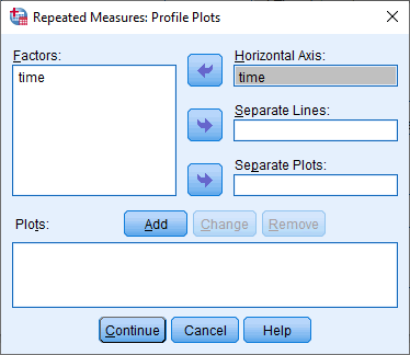
  7. Transfer the within-subjects factor, time, from the Factors: box into the Horizontal Axis: box by clicking on the top right arrow button. You will end up with the following screen:
    'Repeated Measures: Profile Plots' dialogue box. One-way repeated measures ANOVA in SPSS. 'time' transferred

    Published with written permission from SPSS Statistics, IBM Corporation.

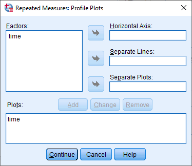
  8. Click on the Add button. This will transfer "time" from the Horizontal Axis: box to the Plots: box, as shown below:
    'Repeated Measures: Profile Plots' dialogue box. One-way repeated measures ANOVA in SPSS. 'time' added to 'Plots' box

    Published with written permission from SPSS Statistics, IBM Corporation.

  9. Click on the Continue button and you will be returned to the Repeated Measures dialogue box.
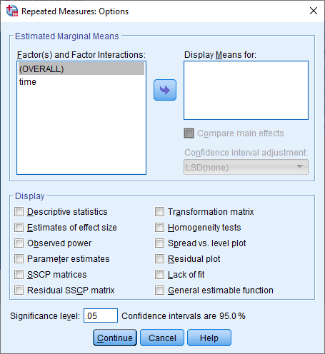
  10. Click on the Options button and you will be presented with the Repeated Measures: Options dialogue box, as shown below:
    'Repeated Measures: Options' dialogue box. One-way repeated measures ANOVA in SPSS. 'time' on the left

    Published with written permission from SPSS Statistics, IBM Corporation.

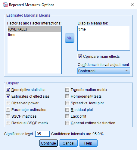
  11. Transfer time from the Factor(s) and Factor Interactions: box to the Display Means for: box using the right arrow button. This will activate the Compare main effects checkbox (i.e., it will no longer be greyed out). Tick this checkbox and select Bonferroni from the drop-down menu under Confidence interval adjustment:. Next, in the –Display– area, tick the Descriptive statistics and Estimates of effect size checkboxes. You will be presented with the following screen:
    'Repeated Measures: Options' dialogue box. One-way repeated measures ANOVA in SPSS. 'time' transferred & options selected

    Published with written permission from SPSS Statistics, IBM Corporation.

  12. Click on the Continue button and you will be returned to the Repeated Measures dialogue box.
  13. Click on the OK button. This will generate the output.
Testimonials
TAKE THE TOUR


SPSS Statistics

SPSS Statistics Output of the Repeated Measures ANOVA

SPSS Statistics generates quite a few tables in its repeated measures ANOVA analysis. In this section, we show you only the main tables required to understand your results from the repeated measures ANOVA. For a complete explanation of the output you have to interpret when checking your data for the five assumptions required to carry out a repeated measures ANOVA, see our enhanced guide. However, in this "quick start" guide, we go through the main tables in turn:

Join the 10,000s of students, academics and professionals who rely on Laerd Statistics.TAKE THE TOUR

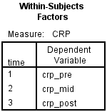
Within-Subjects Factors Table

The Within-Subjects Factors table reminds us of the groups of our independent variable (called a "within-subject factor" in SPSS Statistics) and labels the time points 1, 2 and 3. We will need these labels later on when analysing our results in the Pairwise Comparisons table. Take care not to get confused with the "Dependent Variable" column in this table because it seems to suggest that the different time points are our dependent variable. This is not true – the column label is referring to fact that the dependent variable "CRP" is measured at each of these time points.

'Within-Subjects Factors' table for the one-way repeated measures ANOVA in SPSS Statistics. 3 time points listed & labelled

Published with written permission from SPSS Statistics, IBM Corporation.


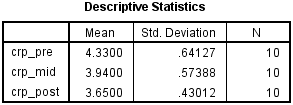
Descriptive Statistics Table

The Descriptive Statistics table simply provides important descriptive statistics for this analysis, as shown below:

'Descriptive Statistics' table. One-way repeated measures ANOVA in SPSS. 'Mean', 'Std. Deviation' & 'N' for each time point

Published with written permission from SPSS Statistics, IBM Corporation.


Tests of Within-Subjects Effects Table

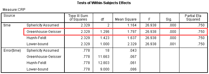
The Tests of Within-Subjects Effects table tells us if there was an overall significant difference between the means at the different time points.

'Tests of Within-Subjects Effects' table. One-way repeated measures ANOVA in SPSS. 'Greenhouse-Geisser' row highlighted

Published with written permission from SPSS Statistics, IBM Corporation.

From this table we are able to discover the F value for the "time" factor, its associated significance level and effect size ("Partial Eta Squared"). As our data violated the assumption of sphericity, we look at the values in the "Greenhouse-Geisser" row (as indicated in red in the screenshot). We can report that when using an ANOVA with repeated measures with a Greenhouse-Geisser correction, the mean scores for CRP concentration were statistically significantly different (F(1.296, 11.663) = 26.938, p < .0005).

Pairwise Comparisons Table

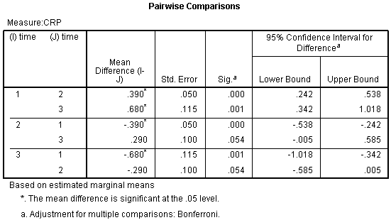
The results presented in the previous table informed us that we have an overall significant difference in means, but we do not know where those differences occurred. This table presents the results of the Bonferroni post hoc test, which allows us to discover which specific means differed. Remember, if your overall ANOVA result was not significant, you should not examine the Pairwise Comparisons table.

'Pairwise Comparisons' table with 'Mean Difference (I-J)', 'Sig. a' & '95% CI for Difference a'. Repeated measures ANOVA SPSS

Published with written permission from SPSS Statistics, IBM Corporation.

Looking at the table above, we need to remember the labels associated with the time points in our experiment from the Within-Subject Factors table. This table gives us the significance level for differences between the individual time points. We can see that there was a statistically significant difference in CRP concentration pre-intervention compared to 3 months into the intervention (p < .0005), and from pre-intervention to post-intervention (p = .001), but no significantly significant difference from 3 months into the intervention compared to post-intervention (p = .054). From the "Mean Difference (I-J)" column we can see that CRP concentration was significantly reduced at this time point.

It is also possible to run comparisons between specific time points that you decided were of interest before you looked at your results. For example, you might have expressed an interest in knowing the difference in CRP concentration between the pre- and post-intervention time points. This type of comparison is often called a planned contrast or a planned simple contrast. However, you do not have to confine yourself to the comparison between two time points only. You might have had an interest in understanding the difference in CRP between the pre-intervention time point and the average of the mid- and post-intervention time points. This is called a complex contrast. All these types of planned contrast are available in SPSS Statistics. In our enhanced guide we show you how to run contrasts in SPSS Statistics using syntax and how to interpret and report the results. In addition, we also show how to "trick" SPSS Statistics into applying a Bonferroni adjustment for multiple comparisons which it would otherwise not do.

Profile Plot

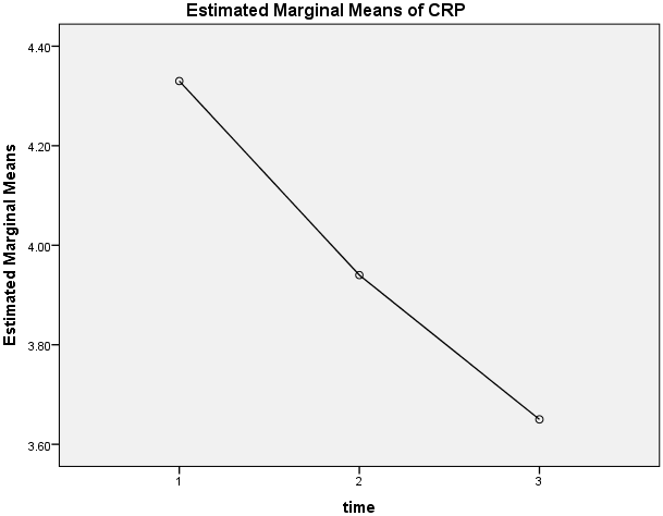
This plot is the last element to this analysis. We are only including it so that you can see some of the limitations of doing so in its current format. You can change many features/properties of a graph's axes using SPSS Statistics. This is important because these profile plots always tend to exaggerate the differences between means by choosing a y-axis range of values that is too narrow. In this case, it is known that most people have CRP concentrations ranging from 0 to 3, so the profile plot that you should produce should take this into consideration. However, this plot can be useful in gaining an easy understanding of the tabular results.

'Estimated Marginal Means of CRP' profile plot for the one-way repeated measures ANOVA in SPSS Statistics

Published with written permission from SPSS Statistics, IBM Corporation.

SPSS Statistics

Reporting the Output

A repeated measures ANOVA with a Greenhouse-Geisser correction determined that mean CRP concentration differed statistically significantly between time points (F(1.298, 11.663) = 26.938, P < 0.0005). Post hoc analysis with a Bonferroni adjustment revealed that CRP concentration was statistically significantly decreased from pre-intervention to three months (0.39 (95% CI, 0.24 to 0.54) mg/L, p < .0005), and from pre-intervention to post-intervention (0.68 (95% CI, 0.34 to 1.02) mg/L, p = .001), but not from three months to post-intervention (0.29 (95% CI, -0.01 to 0.59) mg/L, p = .054).

In our enhanced repeated measures ANOVA guide, we show you how to write up the results from your assumptions tests, repeated measures ANOVA and post hoc results if you need to report this in a dissertation/thesis, assignment or research report. We do this using the Harvard and APA styles. You can learn more about our enhanced content on our Features: Overview page.

Join the 10,000s of students, academics and professionals who rely on Laerd Statistics.TAKE THE TOUR
« prev