Binomial Logistic Regression using SPSS Statistics
Introduction
A binomial logistic regression (often referred to simply as logistic regression), predicts the probability that an observation falls into one of two categories of a dichotomous dependent variable based on one or more independent variables that can be either continuous or categorical. If, on the other hand, your dependent variable is a count, see our Poisson regression guide. Alternatively, if you have more than two categories of the dependent variable, see our multinomial logistic regression guide.
For example, you could use binomial logistic regression to understand whether exam performance can be predicted based on revision time, test anxiety and lecture attendance (i.e., where the dependent variable is "exam performance", measured on a dichotomous scale – "passed" or "failed" – and you have three independent variables: "revision time", "test anxiety" and "lecture attendance"). Alternately, you could use binomial logistic regression to understand whether drug use can be predicted based on prior criminal convictions, drug use amongst friends, income, age and gender (i.e., where the dependent variable is "drug use", measured on a dichotomous scale – "yes" or "no" – and you have five independent variables: "prior criminal convictions", "drug use amongst friends", "income", "age" and "gender").
This "quick start" guide shows you how to carry out binomial logistic regression using SPSS Statistics, as well as interpret and report the results from this test. However, before we introduce you to this procedure, you need to understand the different assumptions that your data must meet in order for binomial logistic regression to give you a valid result. We discuss these assumptions next.
SPSS Statistics
Assumptions
When you choose to analyse your data using binomial logistic regression, part of the process involves checking to make sure that the data you want to analyse can actually be analysed using a binomial logistic regression. You need to do this because it is only appropriate to use a binomial logistic regression if your data "passes" seven assumptions that are required for binomial logistic regression to give you a valid result. In practice, checking for these seven assumptions just adds a little bit more time to your analysis, requiring you to click a few more buttons in SPSS Statistics when performing your analysis, as well as think a little bit more about your data, but it is not a difficult task.
Before we introduce you to some of these assumptions, do not be surprised if, when analysing your own data using SPSS Statistics, one or more of these assumptions is violated (i.e., not met). This is not uncommon when working with real-world data rather than textbook examples, which often only show you how to carry out binomial logistic regression when everything goes well! However, don’t worry. Even when your data fails certain assumptions, there is often a solution to overcome this. First, let's take a look at some of these assumptions:
- Assumption #1: Your dependent variable should be measured on a dichotomous scale. Examples of dichotomous variables include gender (two groups: "males" and "females"), presence of heart disease (two groups: "yes" and "no"), personality type (two groups: "introversion" or "extroversion"), body composition (two groups: "obese" or "not obese"), and so forth. However, if your dependent variable was not measured on a dichotomous scale, but a continuous scale instead, you will need to carry out multiple regression, whereas if your dependent variable was measured on an ordinal scale, ordinal regression would be a more appropriate starting point.
- Assumption #2: You have one or more independent variables, which can be either continuous (i.e., an interval or ratio variable) or categorical (i.e., an ordinal or nominal variable). Examples of continuous variables include revision time (measured in hours), intelligence (measured using IQ score), exam performance (measured from 0 to 100), weight (measured in kg), and so forth. Examples of ordinal variables include Likert items (e.g., a 7-point scale from "strongly agree" through to "strongly disagree"), amongst other ways of ranking categories (e.g., a 3-point scale explaining how much a customer liked a product, ranging from "Not very much" to "Yes, a lot"). Examples of nominal variables include gender (e.g., 2 groups: male and female), ethnicity (e.g., 3 groups: Caucasian, African American and Hispanic), profession (e.g., 5 groups: surgeon, doctor, nurse, dentist, therapist), and so forth. You can learn more about variables in our article: Types of Variable.
- Assumption #3: You should have independence of observations and the dependent variable should have mutually exclusive and exhaustive categories.
- Assumption #4: There needs to be a linear relationship between any continuous independent variables and the logit transformation of the dependent variable. In our enhanced binomial logistic regression guide, we show you how to: (a) use the Box-Tidwell (1962) procedure to test for linearity; and (b) interpret the SPSS Statistics output from this test and report the results.
You can check assumption #4 using SPSS Statistics. Assumptions #1, #2 and #3 should be checked first, before moving onto assumption #4. We suggest testing these assumptions in this order because it represents an order where, if a violation to the assumption is not correctable, you will no longer be able to use a binomial logistic regression (although you may be able to run another statistical test on your data instead). Just remember that if you do not run the statistical tests on these assumptions correctly, the results you get when running binomial logistic regression might not be valid. This is why we dedicate a number of sections of our enhanced binomial logistic regression guide to help you get this right. You can find out about our enhanced content as a whole on our Features: Overview page, or more specifically, learn how we help with testing assumptions on our Features: Assumptions page.
In the section, Test Procedure in SPSS Statistics, we illustrate the SPSS Statistics procedure to perform a binomial logistic regression assuming that no assumptions have been violated. First, we introduce the example that is used in this guide.
SPSS Statistics
Example
A health researcher wants to be able to predict whether the "incidence of heart disease" can be predicted based on "age", "weight", "gender" and "VO2max" (i.e., where VO2max refers to maximal aerobic capacity, an indicator of fitness and health). To this end, the researcher recruited 100 participants to perform a maximum VO2max test as well as recording their age, weight and gender. The participants were also evaluated for the presence of heart disease. A binomial logistic regression was then run to determine whether the presence of heart disease could be predicted from their VO2max, age, weight and gender. Note: this example and data is fictitious.
SPSS Statistics
Setup in SPSS Statistics
In this example, there are six variables: (1) heart_disease, which is whether the participant has heart disease: "yes" or "no" (i.e., the dependent variable); (2) VO2max, which is the maximal aerobic capacity; (3) age, which is the participant's age; (4) weight, which is the participant's weight (technically, it is their 'mass'); and (5) gender, which is the participant's gender (i.e., the independent variables); and (6) caseno, which is the case number.
Note: The caseno variable is used to make it easy for you to eliminate cases (e.g., "significant outliers", "high leverage points" and "highly influential points") that you have identified when checking for assumptions. It is not used directly in calculations for a binomial logistic regression analysis.
In our enhanced binomial logistic regression guide, we show you how to correctly enter data in SPSS Statistics to run a binomial logistic regression when you are also checking for assumptions. You can learn about our enhanced data setup content on our Features: Data Setup page. Alternately, see our generic, "quick start" guide: Entering Data in SPSS Statistics.
SPSS Statistics
Test Procedure in SPSS Statistics
The 10 steps below show you how to analyse your data using a binomial logistic regression in SPSS Statistics when none of the assumptions in the previous section, Assumptions, have been violated. At the end of these 10 steps, we show you how to interpret the results from your binomial logistic regression. If you are looking for help to make sure your data meets these assumptions, which are required when using a binomial logistic regression, and can be tested using SPSS Statistics, you can learn more in our enhanced guide on our Features: Overview page.
Note: The procedure that follows is identical for SPSS Statistics versions 18 to 28, as well as the subscription version of SPSS Statistics, with version 28 and the subscription version being the latest versions of SPSS Statistics. However, in version 27 and the subscription version, SPSS Statistics introduced a new look to their interface called "SPSS Light", replacing the previous look for versions 26 and earlier versions, which was called "SPSS Standard". Therefore, if you have SPSS Statistics versions 27 or 28 (or the subscription version of SPSS Statistics), the images that follow will be light grey rather than blue. However, the procedure is identical.
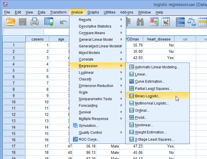
- Click Analyze > Regression > Binary Logistic... on the main menu, as shown below:

Published with written permission from SPSS Statistics, IBM Corporation.
You will be presented with the Logistic Regression dialogue box, as shown below:
Published with written permission from SPSS Statistics, IBM Corporation.
- Transfer the dependent variable, heart_disease, into the Dependent: box, and the independent variables, age, weight, gender and VO2max into the Covariates: box, using the buttons, as shown below:
Published with written permission from SPSS Statistics, IBM Corporation.
Note: For a standard logistic regression you should ignore the and buttons because they are for sequential (hierarchical) logistic regression. The Method: option needs to be kept at the default value, which is . If, for whatever reason, is not selected, you need to change Method: back to . The "Enter" method is the name given by SPSS Statistics to standard regression analysis.
- Click on the button. You will be presented with the Logistic Regression: Define Categorical Variables dialogue box, as shown below:
Published with written permission from SPSS Statistics, IBM Corporation.
Note: SPSS Statistics requires you to define all the categorical predictor values in the logistic regression model. It does not do this automatically.
- Transfer the categorical independent variable, gender, from the Covariates: box to the Categorical Covariates: box, as shown below:
Published with written permission from SPSS Statistics, IBM Corporation.
- In the –Change Contrast– area, change the Reference Category: from the Last option to the First option. Then, click on the button, as shown below:
Published with written permission from SPSS Statistics, IBM Corporation.
Note: Whether you choose Last or First will depend on how you set up your data. In this example, males are to be compared to females, with females acting as the reference category (who were coded "0"). Therefore, First is chosen.
- Click on the button. You will be returned to the Logistic Regression dialogue box.
- Click on the button. You will be presented with the Logistic Regression: Options dialogue box, as shown below:
Published with written permission from SPSS Statistics, IBM Corporation.
- In the –Statistics and Plots– area, click the Classification plots, Hosmer-Lemeshow goodness-of-fit, Casewise listing of residuals and CI for exp(B): options, and in the –Display– area, click the At last step option. You will end up with a screen similar to the one below:
Published with written permission from SPSS Statistics, IBM Corporation.
- Click on the button. You will be returned to the Logistic Regression dialogue box.
- Click on the button. This will generate the output.
SPSS Statistics
Interpreting and Reporting the Output of a Binomial Logistic Regression Analysis
SPSS Statistics generates many tables of output when carrying out binomial logistic regression. In this section, we show you only the three main tables required to understand your results from the binomial logistic regression procedure, assuming that no assumptions have been violated. A complete explanation of the output you have to interpret when checking your data for the assumptions required to carry out binomial logistic regression is provided in our enhanced guide.
However, in this "quick start" guide, we focus only on the three main tables you need to understand your binomial logistic regression results, assuming that your data has already met the assumptions required for binomial logistic regression to give you a valid result:
Variance explained
In order to understand how much variation in the dependent variable can be explained by the model (the equivalent of R2 in multiple regression), you can consult the table below, "Model Summary":
This table contains the Cox & Snell R Square and Nagelkerke R Square values, which are both methods of calculating the explained variation. These values are sometimes referred to as pseudo R2 values (and will have lower values than in multiple regression). However, they are interpreted in the same manner, but with more caution. Therefore, the explained variation in the dependent variable based on our model ranges from 24.0% to 33.0%, depending on whether you reference the Cox & Snell R2 or Nagelkerke R2 methods, respectively. Nagelkerke R2 is a modification of Cox & Snell R2, the latter of which cannot achieve a value of 1. For this reason, it is preferable to report the Nagelkerke R2 value.
Category prediction
Binomial logistic regression estimates the probability of an event (in this case, having heart disease) occurring. If the estimated probability of the event occurring is greater than or equal to 0.5 (better than even chance), SPSS Statistics classifies the event as occurring (e.g., heart disease being present). If the probability is less than 0.5, SPSS Statistics classifies the event as not occurring (e.g., no heart disease). It is very common to use binomial logistic regression to predict whether cases can be correctly classified (i.e., predicted) from the independent variables. Therefore, it becomes necessary to have a method to assess the effectiveness of the predicted classification against the actual classification. There are many methods to assess this with their usefulness often depending on the nature of the study conducted. However, all methods revolve around the observed and predicted classifications, which are presented in the "Classification Table", as shown below:
Firstly, notice that the table has a subscript which states, "The cut value is .500". This means that if the probability of a case being classified into the "yes" category is greater than .500, then that particular case is classified into the "yes" category. Otherwise, the case is classified as in the "no" category (as mentioned previously). Whilst the classification table appears to be very simple, it actually provides a lot of important information about your binomial logistic regression result, including:
- A. The percentage accuracy in classification (PAC), which reflects the percentage of cases that can be correctly classified as "no" heart disease with the independent variables added (not just the overall model).
- B. Sensitivity, which is the percentage of cases that had the observed characteristic (e.g., "yes" for heart disease) which were correctly predicted by the model (i.e., true positives).
- C. Specificity, which is the percentage of cases that did not have the observed characteristic (e.g., "no" for heart disease) and were also correctly predicted as not having the observed characteristic (i.e., true negatives).
- D. The positive predictive value, which is the percentage of correctly predicted cases "with" the observed characteristic compared to the total number of cases predicted as having the characteristic.
- E. The negative predictive value, which is the percentage of correctly predicted cases "without" the observed characteristic compared to the total number of cases predicted as not having the characteristic.
If you are unsure how to interpret the PAC, sensitivity, specificity, positive predictive value and negative predictive value from the "Classification Table", we explain how in our enhanced binomial logistic regression guide.
Variables in the equation
The "Variables in the Equation" table shows the contribution of each independent variable to the model and its statistical significance. This table is shown below:
The Wald test ("Wald" column) is used to determine statistical significance for each of the independent variables. The statistical significance of the test is found in the "Sig." column. From these results you can see that age (p = .003), gender (p = .021) and VO2max (p = .039) added significantly to the model/prediction, but weight (p = .799) did not add significantly to the model. You can use the information in the "Variables in the Equation" table to predict the probability of an event occurring based on a one unit change in an independent variable when all other independent variables are kept constant. For example, the table shows that the odds of having heart disease ("yes" category) is 7.026 times greater for males as opposed to females. If you are unsure how to use odds ratios to make predictions, learn about our enhanced guides on our Features: Overview page.
Putting it all together
Based on the results above, we could report the results of the study as follows (N.B., this does not include the results from your assumptions tests):
A logistic regression was performed to ascertain the effects of age, weight, gender and VO2max on the likelihood that participants have heart disease. The logistic regression model was statistically significant, χ2(4) = 27.402, p < .0005. The model explained 33.0% (Nagelkerke R2) of the variance in heart disease and correctly classified 71.0% of cases. Males were 7.02 times more likely to exhibit heart disease than females. Increasing age was associated with an increased likelihood of exhibiting heart disease, but increasing VO2max was associated with a reduction in the likelihood of exhibiting heart disease.
In addition to the write-up above, you should also include: (a) the results from the assumptions tests that you have carried out; (b) the results from the "Classification Table", including sensitivity, specificity, positive predictive value and negative predictive value; and (c) the results from the "Variables in the Equation" table, including which of the predictor variables were statistically significant and what predictions can be made based on the use of odds ratios. If you are unsure how to do this, we show you in our enhanced binomial logistic regression guide. We also show you how to write up the results from your assumptions tests and binomial logistic regression output if you need to report this in a dissertation/thesis, assignment or research report. We do this using the Harvard and APA styles. You can learn more about our enhanced content on our Features: Overview page.