Multiple Regression Analysis using SPSS Statistics

Introduction

Multiple regression is an extension of simple linear regression. It is used when we want to predict the value of a variable based on the value of two or more other variables. The variable we want to predict is called the dependent variable (or sometimes, the outcome, target or criterion variable). The variables we are using to predict the value of the dependent variable are called the independent variables (or sometimes, the predictor, explanatory or regressor variables).

For example, you could use multiple regression to understand whether exam performance can be predicted based on revision time, test anxiety, lecture attendance and gender. Alternately, you could use multiple regression to understand whether daily cigarette consumption can be predicted based on smoking duration, age when started smoking, smoker type, income and gender.

Multiple regression also allows you to determine the overall fit (variance explained) of the model and the relative contribution of each of the predictors to the total variance explained. For example, you might want to know how much of the variation in exam performance can be explained by revision time, test anxiety, lecture attendance and gender "as a whole", but also the "relative contribution" of each independent variable in explaining the variance.

This "quick start" guide shows you how to carry out multiple regression using SPSS Statistics, as well as interpret and report the results from this test. However, before we introduce you to this procedure, you need to understand the different assumptions that your data must meet in order for multiple regression to give you a valid result. We discuss these assumptions next.

SPSS Statistics

Assumptions

When you choose to analyse your data using multiple regression, part of the process involves checking to make sure that the data you want to analyse can actually be analysed using multiple regression. You need to do this because it is only appropriate to use multiple regression if your data "passes" eight assumptions that are required for multiple regression to give you a valid result. In practice, checking for these eight assumptions just adds a little bit more time to your analysis, requiring you to click a few more buttons in SPSS Statistics when performing your analysis, as well as think a little bit more about your data, but it is not a difficult task.

Before we introduce you to these eight assumptions, do not be surprised if, when analysing your own data using SPSS Statistics, one or more of these assumptions is violated (i.e., not met). This is not uncommon when working with real-world data rather than textbook examples, which often only show you how to carry out multiple regression when everything goes well! However, don’t worry. Even when your data fails certain assumptions, there is often a solution to overcome this. First, let's take a look at these eight assumptions:

• Assumption #1: Your dependent variable should be measured on a continuous scale (i.e., it is either an interval or ratio variable). Examples of variables that meet this criterion include revision time (measured in hours), intelligence (measured using IQ score), exam performance (measured from 0 to 100), weight (measured in kg), and so forth. You can learn more about interval and ratio variables in our article: Types of Variable. If your dependent variable was measured on an ordinal scale, you will need to carry out ordinal regression rather than multiple regression. Examples of ordinal variables include Likert items (e.g., a 7-point scale from "strongly agree" through to "strongly disagree"), amongst other ways of ranking categories (e.g., a 3-point scale explaining how much a customer liked a product, ranging from "Not very much" to "Yes, a lot").
• Assumption #2: You have two or more independent variables, which can be either continuous (i.e., an interval or ratio variable) or categorical (i.e., an ordinal or nominal variable). For examples of continuous and ordinal variables, see the bullet above. Examples of nominal variables include gender (e.g., 2 groups: male and female), ethnicity (e.g., 3 groups: Caucasian, African American and Hispanic), physical activity level (e.g., 4 groups: sedentary, low, moderate and high), profession (e.g., 5 groups: surgeon, doctor, nurse, dentist, therapist), and so forth. Again, you can learn more about variables in our article: Types of Variable. If one of your independent variables is dichotomous and considered a moderating variable, you might need to run a Dichotomous moderator analysis.
• Assumption #3: You should have independence of observations (i.e., independence of residuals), which you can easily check using the Durbin-Watson statistic, which is a simple test to run using SPSS Statistics. We explain how to interpret the result of the Durbin-Watson statistic, as well as showing you the SPSS Statistics procedure required, in our enhanced multiple regression guide.
• Assumption #4: There needs to be a linear relationship between (a) the dependent variable and each of your independent variables, and (b) the dependent variable and the independent variables collectively. Whilst there are a number of ways to check for these linear relationships, we suggest creating scatterplots and partial regression plots using SPSS Statistics, and then visually inspecting these scatterplots and partial regression plots to check for linearity. If the relationship displayed in your scatterplots and partial regression plots are not linear, you will have to either run a non-linear regression analysis or "transform" your data, which you can do using SPSS Statistics. In our enhanced multiple regression guide, we show you how to: (a) create scatterplots and partial regression plots to check for linearity when carrying out multiple regression using SPSS Statistics; (b) interpret different scatterplot and partial regression plot results; and (c) transform your data using SPSS Statistics if you do not have linear relationships between your variables.
• Assumption #5: Your data needs to show homoscedasticity, which is where the variances along the line of best fit remain similar as you move along the line. We explain more about what this means and how to assess the homoscedasticity of your data in our enhanced multiple regression guide. When you analyse your own data, you will need to plot the studentized residuals against the unstandardized predicted values. In our enhanced multiple regression guide, we explain: (a) how to test for homoscedasticity using SPSS Statistics; (b) some of the things you will need to consider when interpreting your data; and (c) possible ways to continue with your analysis if your data fails to meet this assumption.
• Assumption #6: Your data must not show multicollinearity, which occurs when you have two or more independent variables that are highly correlated with each other. This leads to problems with understanding which independent variable contributes to the variance explained in the dependent variable, as well as technical issues in calculating a multiple regression model. Therefore, in our enhanced multiple regression guide, we show you: (a) how to use SPSS Statistics to detect for multicollinearity through an inspection of correlation coefficients and Tolerance/VIF values; and (b) how to interpret these correlation coefficients and Tolerance/VIF values so that you can determine whether your data meets or violates this assumption.
• Assumption #7: There should be no significant outliers, high leverage points or highly influential points. Outliers, leverage and influential points are different terms used to represent observations in your data set that are in some way unusual when you wish to perform a multiple regression analysis. These different classifications of unusual points reflect the different impact they have on the regression line. An observation can be classified as more than one type of unusual point. However, all these points can have a very negative effect on the regression equation that is used to predict the value of the dependent variable based on the independent variables. This can change the output that SPSS Statistics produces and reduce the predictive accuracy of your results as well as the statistical significance. Fortunately, when using SPSS Statistics to run multiple regression on your data, you can detect possible outliers, high leverage points and highly influential points. In our enhanced multiple regression guide, we: (a) show you how to detect outliers using "casewise diagnostics" and "studentized deleted residuals", which you can do using SPSS Statistics, and discuss some of the options you have in order to deal with outliers; (b) check for leverage points using SPSS Statistics and discuss what you should do if you have any; and (c) check for influential points in SPSS Statistics using a measure of influence known as Cook's Distance, before presenting some practical approaches in SPSS Statistics to deal with any influential points you might have.
• Assumption #8: Finally, you need to check that the residuals (errors) are approximately normally distributed (we explain these terms in our enhanced multiple regression guide). Two common methods to check this assumption include using: (a) a histogram (with a superimposed normal curve) and a Normal P-P Plot; or (b) a Normal Q-Q Plot of the studentized residuals. Again, in our enhanced multiple regression guide, we: (a) show you how to check this assumption using SPSS Statistics, whether you use a histogram (with superimposed normal curve) and Normal P-P Plot, or Normal Q-Q Plot; (b) explain how to interpret these diagrams; and (c) provide a possible solution if your data fails to meet this assumption.

You can check assumptions #3, #4, #5, #6, #7 and #8 using SPSS Statistics. Assumptions #1 and #2 should be checked first, before moving onto assumptions #3, #4, #5, #6, #7 and #8. Just remember that if you do not run the statistical tests on these assumptions correctly, the results you get when running multiple regression might not be valid. This is why we dedicate a number of sections of our enhanced multiple regression guide to help you get this right. You can find out about our enhanced content as a whole on our Features: Overview page, or more specifically, learn how we help with testing assumptions on our Features: Assumptions page.

In the section, Procedure, we illustrate the SPSS Statistics procedure to perform a multiple regression assuming that no assumptions have been violated. First, we introduce the example that is used in this guide.

SPSS Statistics

Example

A health researcher wants to be able to predict "VO₂max", an indicator of fitness and health. Normally, to perform this procedure requires expensive laboratory equipment and necessitates that an individual exercise to their maximum (i.e., until they can longer continue exercising due to physical exhaustion). This can put off those individuals who are not very active/fit and those individuals who might be at higher risk of ill health (e.g., older unfit subjects). For these reasons, it has been desirable to find a way of predicting an individual's VO₂max based on attributes that can be measured more easily and cheaply. To this end, a researcher recruited 100 participants to perform a maximum VO₂max test, but also recorded their "age", "weight", "heart rate" and "gender". Heart rate is the average of the last 5 minutes of a 20 minute, much easier, lower workload cycling test. The researcher's goal is to be able to predict VO₂max based on these four attributes: age, weight, heart rate and gender.

SPSS Statistics

Setup in SPSS Statistics

In SPSS Statistics, we created six variables: (1) VO₂max, which is the maximal aerobic capacity; (2) age, which is the participant's age; (3) weight, which is the participant's weight (technically, it is their 'mass'); (4) heart_rate, which is the participant's heart rate; (5) gender, which is the participant's gender; and (6) caseno, which is the case number. The caseno variable is used to make it easy for you to eliminate cases (e.g., "significant outliers", "high leverage points" and "highly influential points") that you have identified when checking for assumptions. In our enhanced multiple regression guide, we show you how to correctly enter data in SPSS Statistics to run a multiple regression when you are also checking for assumptions. You can learn about our enhanced data setup content on our Features: Data Setup page. Alternately, see our generic, "quick start" guide: Entering Data in SPSS Statistics.

SPSS Statistics

Test Procedure in SPSS Statistics

The seven steps below show you how to analyse your data using multiple regression in SPSS Statistics when none of the eight assumptions in the previous section, Assumptions, have been violated. At the end of these seven steps, we show you how to interpret the results from your multiple regression. If you are looking for help to make sure your data meets assumptions #3, #4, #5, #6, #7 and #8, which are required when using multiple regression and can be tested using SPSS Statistics, you can learn more in our enhanced guide (see our Features: Overview page to learn more).

Note: The procedure that follows is identical for SPSS Statistics versions 18 to 28, as well as the subscription version of SPSS Statistics, with version 28 and the subscription version being the latest versions of SPSS Statistics. However, in version 27 and the subscription version, SPSS Statistics introduced a new look to their interface called "SPSS Light", replacing the previous look for versions 26 and earlier versions, which was called "SPSS Standard". Therefore, if you have SPSS Statistics versions 27 or 28 (or the subscription version of SPSS Statistics), the images that follow will be light grey rather than blue. However, the procedure is identical.

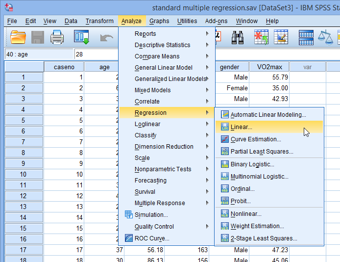
1. Click Analyze > Regression > Linear... on the main menu, as shown below:
   

   Published with written permission from SPSS Statistics, IBM Corporation.

   Note: Don't worry that you're selecting Analyze > Regression > Linear... on the main menu or that the dialogue boxes in the steps that follow have the title, Linear Regression. You have not made a mistake. You are in the correct place to carry out the multiple regression procedure. This is just the title that SPSS Statistics gives, even when running a multiple regression procedure.

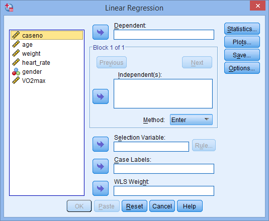
2. You will be presented with the Linear Regression dialogue box below:
   

   Published with written permission from SPSS Statistics, IBM Corporation.

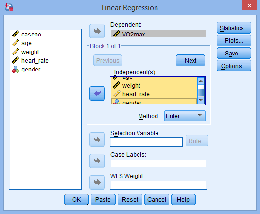
3. Transfer the dependent variable, VO₂max, into the Dependent: box and the independent variables, age, weight, heart_rate and gender into the Independent(s): box, using the buttons, as shown below (all other boxes can be ignored):
   

   Published with written permission from SPSS Statistics, IBM Corporation.

   Note: For a standard multiple regression you should ignore the and buttons as they are for sequential (hierarchical) multiple regression. The Method: option needs to be kept at the default value, which is . If, for whatever reason, is not selected, you need to change Method: back to . The method is the name given by SPSS Statistics to standard regression analysis.

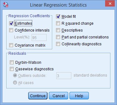
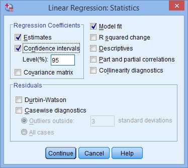
4. Click on the button. You will be presented with the Linear Regression: Statistics dialogue box, as shown below:
   

   Published with written permission from SPSS Statistics, IBM Corporation.

5. In addition to the options that are selected by default, select Confidence intervals in the –Regression Coefficients– area leaving the Level(%): option at "95". You will end up with the following screen:
   

   Published with written permission from SPSS Statistics, IBM Corporation.

6. Click on the button. You will be returned to the Linear Regression dialogue box.
7. Click on the button. This will generate the output.