Measures of Central Tendency
Introduction
A measure of central tendency is a single value that attempts to describe a set of data by identifying the central position within that set of data. As such, measures of central tendency are sometimes called measures of central location. They are also classed as summary statistics. The mean (often called the average) is most likely the measure of central tendency that you are most familiar with, but there are others, such as the median and the mode.
The mean, median and mode are all valid measures of central tendency, but under different conditions, some measures of central tendency become more appropriate to use than others. In the following sections, we will look at the mean, mode and median, and learn how to calculate them and under what conditions they are most appropriate to be used.
Mean (Arithmetic)
The mean (or average) is the most popular and well known measure of central tendency. It can be used with both discrete and continuous data, although its use is most often with continuous data (see our Types of Variable guide for data types). The mean is equal to the sum of all the values in the data set divided by the number of values in the data set. So, if we have \( n \) values in a data set and they have values \( x_1, x_2, \) …\(, x_n \), the sample mean, usually denoted by \( \overline{x} \) (pronounced "x bar"), is:
$$ \overline{x} = {{x_1 + x_2 + \dots + x_n}\over{n}} $$
This formula is usually written in a slightly different manner using the Greek capitol letter, \( \sum \), pronounced "sigma", which means "sum of...":
$$ \overline{x} = {{\sum{x}}\over{n}} $$
You may have noticed that the above formula refers to the sample mean. So, why have we called it a sample mean? This is because, in statistics, samples and populations have very different meanings and these differences are very important, even if, in the case of the mean, they are calculated in the same way. To acknowledge that we are calculating the population mean and not the sample mean, we use the Greek lower case letter "mu", denoted as \( \mu \):
$$ \mu = {{\sum{x}}\over{n}} $$
The mean is essentially a model of your data set. It is the value that is most common. You will notice, however, that the mean is not often one of the actual values that you have observed in your data set. However, one of its important properties is that it minimises error in the prediction of any one value in your data set. That is, it is the value that produces the lowest amount of error from all other values in the data set.
An important property of the mean is that it includes every value in your data set as part of the calculation. In addition, the mean is the only measure of central tendency where the sum of the deviations of each value from the mean is always zero.
When not to use the mean
The mean has one main disadvantage: it is particularly susceptible to the influence of outliers. These are values that are unusual compared to the rest of the data set by being especially small or large in numerical value. For example, consider the wages of staff at a factory below:
| Staff | 1 | 2 | 3 | 4 | 5 | 6 | 7 | 8 | 9 | 10 | | Salary | 15k | 18k | 16k | 14k | 15k | 15k | 12k | 17k | 90k | 95k |
The mean salary for these ten staff is $30.7k. However, inspecting the raw data suggests that this mean value might not be the best way to accurately reflect the typical salary of a worker, as most workers have salaries in the $12k to 18k range. The mean is being skewed by the two large salaries. Therefore, in this situation, we would like to have a better measure of central tendency. As we will find out later, taking the median would be a better measure of central tendency in this situation.
Another time when we usually prefer the median over the mean (or mode) is when our data is skewed (i.e., the frequency distribution for our data is skewed). If we consider the normal distribution - as this is the most frequently assessed in statistics - when the data is perfectly normal, the mean, median and mode are identical. Moreover, they all represent the most typical value in the data set. However, as the data becomes skewed the mean loses its ability to provide the best central location for the data because the skewed data is dragging it away from the typical value. However, the median best retains this position and is not as strongly influenced by the skewed values. This is explained in more detail in the skewed distribution section later in this guide.
Median
The median is the middle score for a set of data that has been arranged in order of magnitude. The median is less affected by outliers and skewed data. In order to calculate the median, suppose we have the data below:
We first need to rearrange that data into order of magnitude (smallest first):
Our median mark is the middle mark - in this case, 56 (highlighted in bold). It is the middle mark because there are 5 scores before it and 5 scores after it. This works fine when you have an odd number of scores, but what happens when you have an even number of scores? What if you had only 10 scores? Well, you simply have to take the middle two scores and average the result. So, if we look at the example below:
We again rearrange that data into order of magnitude (smallest first):
Only now we have to take the 5th and 6th score in our data set and average them to get a median of 55.5.
Mode
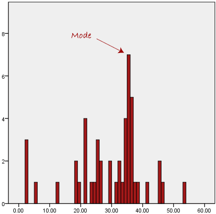
The mode is the most frequent score in our data set. On a histogram it represents the highest bar in a bar chart or histogram. You can, therefore, sometimes consider the mode as being the most popular option. An example of a mode is presented below:

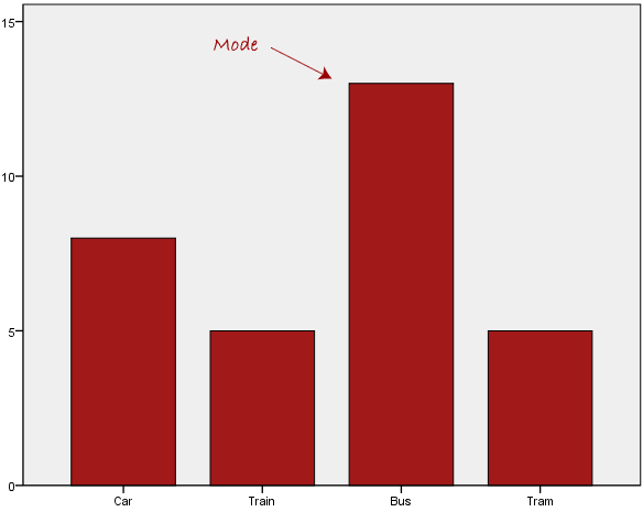
Normally, the mode is used for categorical data where we wish to know which is the most common category, as illustrated below:
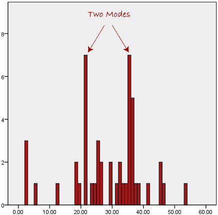
We can see above that the most common form of transport, in this particular data set, is the bus. However, one of the problems with the mode is that it is not unique, so it leaves us with problems when we have two or more values that share the highest frequency, such as below:
We are now stuck as to which mode best describes the central tendency of the data. This is particularly problematic when we have continuous data because we are more likely not to have any one value that is more frequent than the other. For example, consider measuring 30 peoples' weight (to the nearest 0.1 kg). How likely is it that we will find two or more people with exactly the same weight (e.g., 67.4 kg)? The answer, is probably very unlikely - many people might be close, but with such a small sample (30 people) and a large range of possible weights, you are unlikely to find two people with exactly the same weight; that is, to the nearest 0.1 kg. This is why the mode is very rarely used with continuous data.
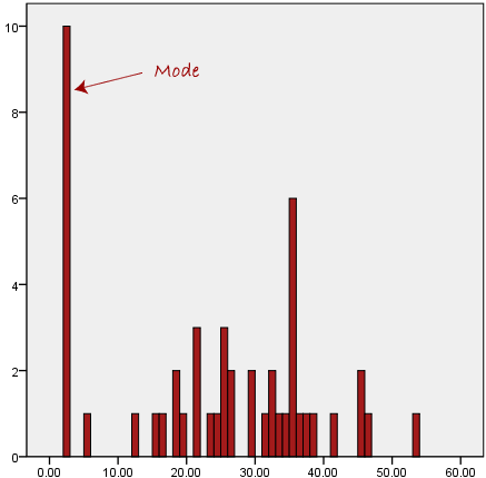
Another problem with the mode is that it will not provide us with a very good measure of central tendency when the most common mark is far away from the rest of the data in the data set, as depicted in the diagram below:
In the above diagram the mode has a value of 2. We can clearly see, however, that the mode is not representative of the data, which is mostly concentrated around the 20 to 30 value range. To use the mode to describe the central tendency of this data set would be misleading.
Skewed Distributions and the Mean and Median
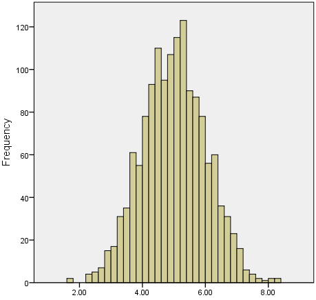
We often test whether our data is normally distributed because this is a common assumption underlying many statistical tests. An example of a normally distributed set of data is presented below:
When you have a normally distributed sample you can legitimately use both the mean or the median as your measure of central tendency. In fact, in any symmetrical distribution the mean, median and mode are equal. However, in this situation, the mean is widely preferred as the best measure of central tendency because it is the measure that includes all the values in the data set for its calculation, and any change in any of the scores will affect the value of the mean. This is not the case with the median or mode.
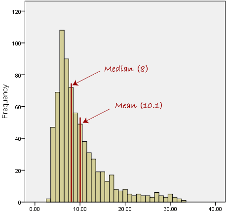
However, when our data is skewed, for example, as with the right-skewed data set below:
We find that the mean is being dragged in the direct of the skew. In these situations, the median is generally considered to be the best representative of the central location of the data. The more skewed the distribution, the greater the difference between the median and mean, and the greater emphasis should be placed on using the median as opposed to the mean. A classic example of the above right-skewed distribution is income (salary), where higher-earners provide a false representation of the typical income if expressed as a mean and not a median.
If dealing with a normal distribution, and tests of normality show that the data is non-normal, it is customary to use the median instead of the mean. However, this is more a rule of thumb than a strict guideline. Sometimes, researchers wish to report the mean of a skewed distribution if the median and mean are not appreciably different (a subjective assessment), and if it allows easier comparisons to previous research to be made.
Summary of when to use the mean, median and mode
Please use the following summary table to know what the best measure of central tendency is with respect to the different types of variable.
| Type of Variable | Best measure of central tendency |
| Nominal | Mode |
| Ordinal | Median |
| Interval/Ratio (not skewed) | Mean |
| Interval/Ratio (skewed) | Median |
For answers to frequently asked questions about measures of central tendency, please go the next page.