SPSS Statistics
Example used in this guide
A firm will be launching a new product and hires an advertising agency to create a TV advert that it hopes will encourage people to purchase its new product. The firm is quite traditional and usually runs TV adverts that are very conservative. However, the firm wants the advertising agency to design two TV adverts: one "conservative" and one "edgy" (i.e., more modern). The firm does not know whether the "conservative" TV advert or the "edgy" TV advert will encourage more people to purchase their new product. However, the firm is curious to see the effect that the "edgy" TV advert has on potential customers. Therefore, the firm asks the advertising agency to test whether a sample of potential customers prefer the "conservative" or "edgy" TV advert. The firm will use this information to decide whether to run the "conservative" TV advert or the "edgy" TV advert.
After the advertising agency creates these two TV adverts, they are shown to a random sample of 23 potential customers. For the purpose of running a binomial test, one of the two TV adverts has to be selected as the "success" category. Since the advertising agency knows that the firm is particularly curious about the effect that the "edgy" TV advert might have on potential customers, the advertising agency selects the "edgy" TV advert as the "success" category.
Explanation: Whilst the advertising agency chose the "edgy" TV advert as the "success" category, the choice of "success" category is arbitrary, meaning that it does not matter which category is selected for this type of study design (i.e., theoretically, the "success" of either category is equal; that is, 50:50 or 50% as likely). Therefore, the advertising agency could have selected the "conservative" TV advert as the "success" category instead, or even waited until after the data had been collected to see which of the two TV adverts – "edgy" or "conservative" – had the largest proportion, and then selected the category with the largest proportion as the "success" category).
Using the sample of 23 potential customers, the binomial test determines whether the proportion of potential customers who prefer the "edgy" TV advert is different to/not the same as the proportion of potential customers who prefer the "conservative" TV advert. In other words, the binomial test will determine whether the two categories – "edgy" and "conservative" – are not equally distributed in the population of all potential customers (as opposed to just the sample of 23 potential customers). It does this by determining whether the proportion of 23 potential customers who prefer the "edgy" TV advert comes from a population of all potential customers with a theoretical/hypothesized proportion of 0.5 (i.e., where "0.5" indicates that the two TV adverts equally encourage potential customers to purchase the new product, which can also be expressed as 50:50, a 50% chance of selecting either of the two TV adverts, or a proportion of 0.5).
Therefore, in the example we are using to demonstrate a binomial test and corresponding 95% confidence interval (CI) in this introductory guide, the dichotomous response variable is advert_type, which has two categories: "edgy" and "conservative". In the next section, we explain how to set up your data in SPSS Statistics to run a binomial test and corresponding 95% CI using this dichotomous response variable: advert_type.
SPSS Statistics
Data setup in SPSS Statistics when carrying out a binomial test and corresponding 95% confidence interval (CI)
To carry out a binomial test and corresponding 95% CI, you have to set up one variable in SPSS Statistics. In this example, this is the dichotomous response variable, advert_type, which has two categories – "edgy" and "conservative" – to reflect the 23 potential customers who were asked to state which of two TV adverts – an "edgy" TV advert and a "conservative" TV advert – they prefer in terms of encouraging them to purchase a new product.
To set up this variable, SPSS Statistics has a Variable View where you define the types of variables you are analysing and a Data View where you enter your data for these variables. First, we show you how to set up a dichotomous response variable in the Variable View window of SPSS Statistics. Next, we show you how to enter your data into the Data View window.
The "Variable View" in SPSS Statistics
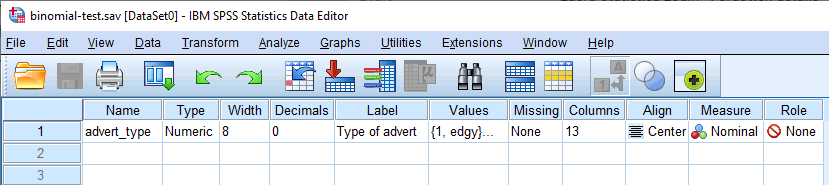
At the end of the data setup process, your Variable View window will look like the one below, which illustrates the setup for the dichotomous response variable, advert_type:

Published with written permission from SPSS Statistics, IBM Corporation.
In the Variable View window above, you will have entered one variable. In our example, the dichotomous response variable, advert_type, is displayed on row .
The name of your dichotomous response variable should be entered in the cell under the column (e.g., "tv_advert" in row to represent our dichotomous response variable, advert_type). There are certain "illegal" characters that cannot be entered into the cell. Therefore, if you get an error message and you would like us to add an SPSS Statistics guide to explain what these illegal characters are, please contact us.
Note: For your own clarity, you can also provide a label for your variable in the column. For example, the label we entered for "tv_advert" was "Type of TV advert".
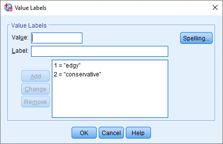
The cell under the column should contain the information about the categories of your dichotomous response variable (e.g., "edgy" and "conservative" for advert_type). To enter this information, click into the cell under the column for your dichotomous response variable. The button will appear in the cell. Click on this button and the Value Labels dialogue box will appear. You now need to give each category of your dichotomous response variable a "value", which you enter into the Value: box (e.g., "1"), as well as a "label", which you enter into the Label: box (e.g., "edgy"). By clicking on the button the coding will appear in the main box (e.g., "1.00 = "edgy" for advert_type). The setup for our dichotomous response variable is shown in the Value Labels dialogue box below:
Published with written permission from SPSS Statistics, IBM Corporation.
Note: You will typically enter an integer (e.g., "1") into the Value: box to represent the categories of your nominal (dichotomous) variable and not a decimal (e.g., "1.00"). However, SPSS Statistics adds the 2 decimal places by default when you click on the button (e.g., 1.00 = "edgy"). Therefore, you can simply click into the cells under the column and change these to "0" using the arrows, which is why "edgy" is coded as "1" and not "1.00" in the Value Labels box above. Therefore, do not think that you have done anything wrong if 2 decimals places have been added to the values you set up in the Value Labels box.
The cell under the column should show , indicating that you have dichotomous (nominal) variable (e.g., advert_type, as in our example). Finally, the cell under the column should show .
Note: We suggest changing the cell under the column from to , but you do not have to make this change. We suggest that you do because there are certain analyses in SPSS Statistics where the setting results in your variables being automatically transferred into certain fields of the dialogue boxes you are using. Since you may not want to transfer these variables, we suggest changing the setting to so that this does not happen automatically.
You have now successfully entered all the information that SPSS Statistics needs to know about your dichotomous response variable into the Variable View window. In the next section, we show you how to enter your data into the Data View window.
The Data View in SPSS Statistics
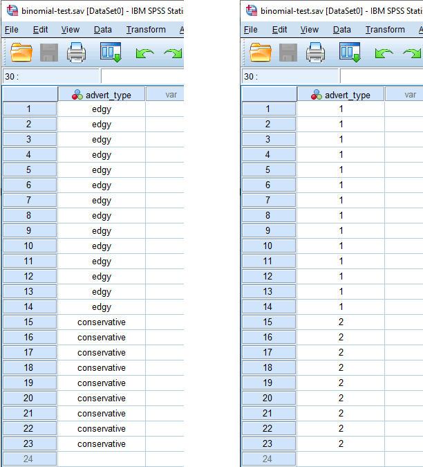
Based on the file setup for the dichotomous response variable in the Variable View window above, the Data View window should look as follows:
Published with written permission from SPSS Statistics, IBM Corporation.
On the left above, the responses for our dichotomous response variable are shown in text (e.g., "edgy" and "conservative" under the column). On the right, the same responses for our dichotomous response variable are shown using its underlying coding (i.e., "1" and "2" under the column). This reflects the coding in the Value Labels dialogue box: "1" = "edgy" and "2" = "conservative" for our dichotomous response variable, advert_type. You can toggle between these two views of your data by clicking the "Value Labels" icon () in the main toolbar.
Now, you simply have to enter your data into the cells under each column. Remember that each row represents one case (e.g., one case in our example represents one potential customer). For example, in row , our first case was a potential customer who stated that they preferred the "edgy " TV advert. As another example, in row , our 15th case was a potential customer who stated that they preferred the "conservative" TV advert.
Since these cells will initially be empty, you need to click into the cells to enter your data. You will notice that when you click into the cells under your dichotomous response variable, SPSS Statistics will give you a drop-down option with the two categories – "1" or edgy" and "2" or "conservative" – already populated.
Your data is now set up correctly in SPSS Statistics. In the next section, we show you how to carry out a binomial test and corresponding 95% CI using SPSS Statistics.
SPSS Statistics
SPSS Statistics procedure to carry out a binomial test and corresponding 95% confidence interval (CI)
The 10 steps below show you how to analyse your data using an exact binomial test and corresponding exact Clopper-Pearson 95% CI procedure in SPSS Statistics. The exact binomial test is automatically carried out in SPSS Statistics when you have a small sample size (as determined by SPSS Statistics), as we do in our example. These 10 steps are the same for SPSS Statistics versions 18 to 30, where the latest versions of SPSS Statistics are version 30 and the subscription version. If you are unsure which version of SPSS Statistics you are using, see our guide: Identifying your version of SPSS Statistics.
Note: We demonstrate how to carry out a binomial test and corresponding 95% CI using the exact binomial test and corresponding exact Clopper-Pearson 95% CI. However, there are many different types of test and procedures that you can use. Whilst we demonstrate the exact Clopper-Pearson 95% CI since this is available in SPSS Statistics, it is not necessarily the best test or confidence interval to use. Therefore, we will be adding a guide to demonstrate superior methods using R (and RStudio). If you would like us to let you know when we add this guide to the site, please contact us
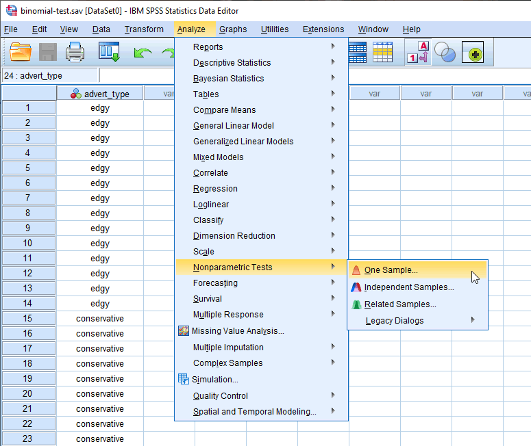
- Click Nonparametric Tests > One Sample... on the main menu:
Published with written permission from SPSS Statistics, IBM Corporation.
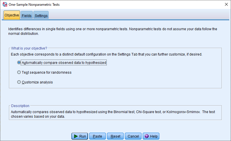
You will be presented with the One-Sample Nonparametric Tests dialogue box, as shown below:
Published with written permission from SPSS Statistics, IBM Corporation.
- In the –What is your objective?– area, select Customize analysis, as shown below:
Published with written permission from SPSS Statistics, IBM Corporation.
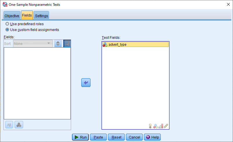
- Click on the tab and you will be presented with the following screen:
Published with written permission from SPSS Statistics, IBM Corporation.
- Transfer the dichotomous response variable, advert_type, from the Fields: box into the Test Fields: box. To do this, highlight the variable and use the button to move it into the Test Fields: box. You will end up with the following screen:
Published with written permission from SPSS Statistics, IBM Corporation.
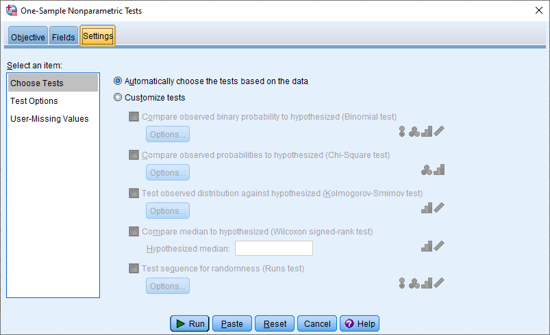
- Click on the tab and you will be presented with the following screen:
Published with written permission from SPSS Statistics, IBM Corporation.
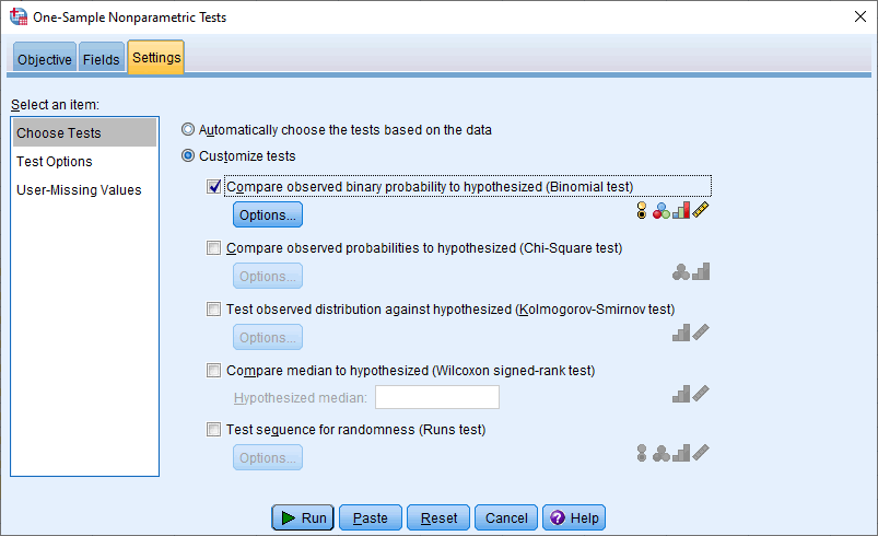
- Click on Customize tests and then Compare observed binary probability to hypothesized (Binomial test), which will activate the button, as shown below:
Published with written permission from SPSS Statistics, IBM Corporation.
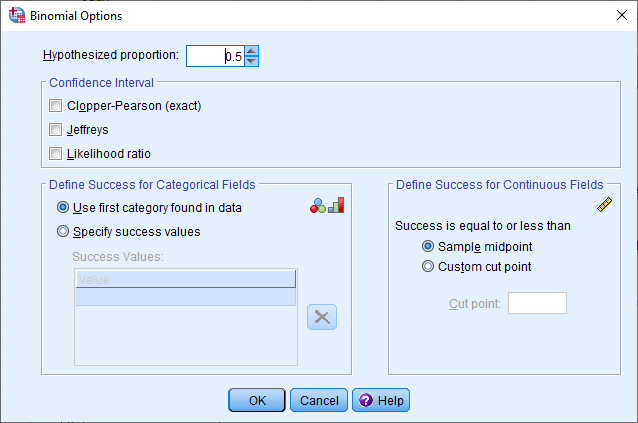
- Click on the button. You will be presented with the Binomial Options dialogue box, as shown below:
Published with written permission from SPSS Statistics, IBM Corporation.
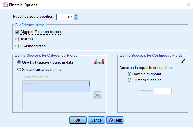
- In the –Confidence Interval– area, select Clopper-Pearson (exact), as shown below:
Published with written permission from SPSS Statistics, IBM Corporation.
- Click on the button and you will be returned to the One-Sample Nonparametric Tests dialogue box.
- Click on the button to generate the output for the exact binomial test and corresponding exact Clopper-Pearson 95% CI procedure. This will be displayed in the IBM SPSS Statistics Viewer.
The results from the binomial test analysis above are discussed in the next section: Interpreting the results of a binomial test analysis.
SPSS Statistics
Interpreting the results of a binomial test analysis and corresponding 95% confidence interval (CI)
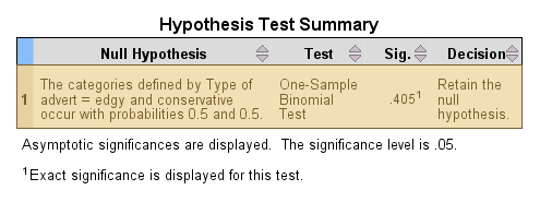
After carrying out an exact binomial test and exact Clopper-Pearson 95% CI in the previous section, SPSS Statistics displays the results in its IBM SPSS Statistics Viewer, starting with the Hypothesis Test Summary table, as shown below:
Published with written permission from SPSS Statistics, IBM Corporation.
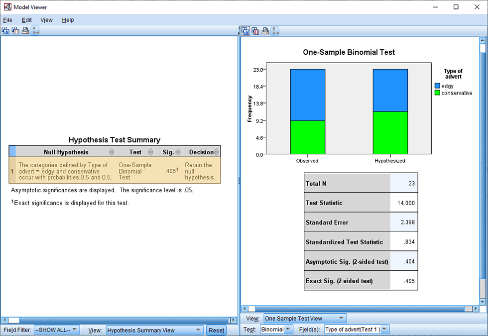
In order to view all of the results from the exact binomial test and exact Clopper-Pearson 95% CI, you need to double-click on this Hypothesis Test Summary table, which will launch SPSS Statistics' Model Viewer in a separate window, as shown below:
Note: The Model Viewer is the default display in SPSS Statistics when carrying out an exact binomial test and exact Clopper-Pearson 95% CI. However, if you have changed the display options in SPSS Statistics (i.e., via the main menu under Edit > Options...) from the Model Viewer to Pivot tables and charts, all of the results will be displayed in the initial IBM SPSS Statistics Viewer instead. However, even though the location where the results are displayed is different, the tables produced are the same.
Published with written permission from SPSS Statistics, IBM Corporation.
The Model Viewer includes three tables – the Hypothesis Test Summary table, the One-Sample Binomial Test table and the Confidence Interval Summary table – as well as one of two bar charts that you will refer to, which is displayed in the Categorical Field Information area. In this introductory guide, we explain the results from the exact binomial test and exact Clopper-Pearson 95% CI binomial test that was carried out in the previous section, using these three tables and bar chart.
The "Hypothesis Test Summary" table
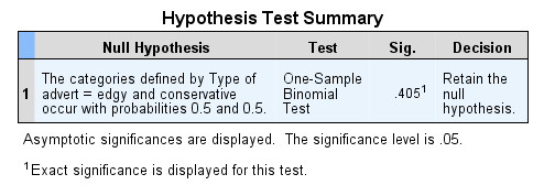
The Hypothesis Test Summary table displayed in the IBM SPSS Statistics Viewer is also displayed in the left-hand pane of the Model Viewer above, as shown below:
Note: The Hypothesis Test Summary table below may look a little different from the one in the IBM SPSS Statistics Viewer, which was shown at the beginning of this section. However, the content in the table is the same. SPSS Statistics simply changes the colour of the table based on whether the result of the binomial test is statistically significant, which we discuss in this section. Therefore, if the colour of your Hypothesis Test Summary table is different from the one below, this does not indicate that you have run the procedure in the previous section incorrectly.
Published with written permission from SPSS Statistics, IBM Corporation.
Note: The Hypothesis Test Summary table is shown in the left-hand pane when you first launch the Model Viewer. However, if it is not displayed, select from the drop-down options in the View: box or click on the button.
The Hypothesis Test Summary table provides the p-value of the exact binomial test under the "Sig." column, which in our example is .405 (i.e., p = .405). SPSS Statistics does not always produce an exact p-value. Sometimes it will produce an asymptotic p-value (a non-exact p-value). An exact p-value is only calculated if your data is considered small enough/sufficiently small to warranty this calculation based on criteria defined by SPSS Statistics. You can tell which type of p-value calculation SPSS Statistics has made by consulting the Hypothesis Test Summary table to see if a sub-note has been added that states, "Exact significance is displayed for this test". In this example, this sub-note is present so an exact p-value is being displayed. This information is also replicated in the One-Sample Binomial Test table, discussed in the next section.
The "One-Sample Binomial Test" table
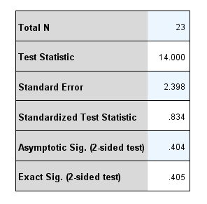
The One-Sample Binomial Test table, shown below, includes a number of results that are useful when interpreting and reporting the results from a binomial test:
Published with written permission from SPSS Statistics, IBM Corporation.
Note: The Hypothesis Test Summary table is shown in the right-hand pane when you first launch the Model Viewer. However, if it is not displayed, select from the drop-down options in the View: box.
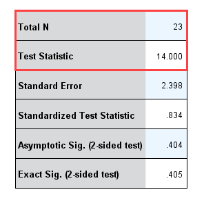
The first two useful pieces of information are found in the first two rows – the "Total N" and "Test Statistic" rows – as highlighted below:
Published with written permission from SPSS Statistics, IBM Corporation.
The first row, "Total N", indicates the total sample size that was used in the calculations of the binomial test, which in this case was "23", reflecting the 23 potential customers who took part in the research. It is useful to check this row simply to make sure that the number of cases included in the analysis (i.e., where the "cases" in our study are the potential customers) is what you expect, to make sure that no cases were excluded unexpectedly from your analysis.
The second row informs you of the number of cases (i.e., potential customers in this example) that were in the category you defined as the "success" category, which in our example reflects those potential customers who preferred the "edgy" TV advert. As a reminder, we discussed the need to choose a "success" category in order to run a binomial test and our choice of the "edgy" TV advert as our "success" category in the section: Example used in this guide. As such, since the "Test Statistics" was 14.000, we know that 14 potential customers preferred the "edgy" TV advert (i.e., 14 out of 23 potential customers preferred the "edgy" TV advert). This is also highlighted in the bar chart entitled Categorical Field Information, as shown below, where the Total N = 23 and the "Type of advert=edgy" shows N=14, which is 60.9% of cases (i.e., 14 ÷ 23 = 60.9% to 1 decimal place):
Published with written permission from SPSS Statistics, IBM Corporation.
Note: To display the bar chart above, select from the drop-down options in the View: box. The bar chart will be displayed in the right-hand pane of the Model Viewer.
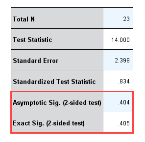
You can also see that two statistical significance values (i.e., two p-values) for the binomial test are displayed in last two rows of the One-Sample Binomial Test table: the asymptotic (2-sided) p-value along the "Asymptotic Sig.(2-sided test)" row and the exact (2-sided) p-value along the Exact Sig.(2-sided test)" row, as highlighted below:
Published with written permission from SPSS Statistics, IBM Corporation.
As stated before, SPSS Statistics will only display an exact (2-sided) p-value if it considers your sample size to be sufficiently small to run an exact binomial test. The exact p-value is used in this example, which is .405 (i.e., p = .405). Whilst the p-value is useful, it is the exact Clopper-Pearson 95% CI procedure discussed in the next section that is usually of most importance when analysing your results.
The "Confidence Interval Summary" table
To display the Confidence Interval Summary table, select from the drop-down options in the View: box. The Confidence Interval Summary table, shown below, will be displayed in the left-hand pane of the Model Viewer:
Published with written permission from SPSS Statistics, IBM Corporation.
The first two useful pieces of information are found under the first two columns – "Confidence Interval Type" and "Parameter" rows – as highlighted below:
Published with written permission from SPSS Statistics, IBM Corporation.
The information in the brackets ( ) after the text, "One-Sample Binomial Success Rate", displayed under the "Confidence Interval Type" column, indicates the type of confidence interval (CI) procedure that was selected in Step 8 of the procedure we carried out in the previous section. Since we choose to use an exact Clopper-Pearson 95% CI procedure, these brackets ( ) include the words "Clopper-Pearson".
Furthermore, the information in the brackets ( ) after the word, "Probability", displayed under the "Parameter" column, indicates which category of your dichotomous response variable acted as the "success" category when calculating the exact Clopper-Pearson 95% CI. Since we choose the "edgy" category as our "success" category, the word "edgy" is displayed after the name of our dichotomous response variable, "Type of advert", under the "Parameter" column (i.e., "Type of advert=edgy").
These two pieces of information are useful simply to confirm that you have: (a) carried out the correct type of confidence interval; and (b) used the correct "success" category (i.e., by "correct", we mean the type of confidence interval and "success" category that you wanted to use).
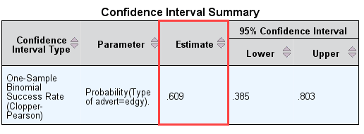
The next column, "Estimate", shows the proportion of potential customers that preferred the "edgy" TV advert rather than the "conservative" TV advert (i.e., were more likely to make a purchase when viewing the "edgy" TV advert), as highlighted below:
Published with written permission from SPSS Statistics, IBM Corporation.
The proportion in the "Estimate" column is .609, which can also be expressed as 60.9% (i.e., .609 x 100 = 60.9%).
This is the proportion in the sample of 23 potential customers, but also the estimate of the proportion in the population (i.e., all potential customers). In other words, it is estimated that 60.9% of all potential customers would prefer the "edgy" TV advert.
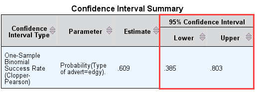
Since this estimate is based on a single sample (i.e., the 23 potential customers in this study), there will be some uncertainty in its value. Therefore, the 95% confidence interval (CI) calculated using the exact Clopper-Pearson method can provide a range of values that the population proportion (i.e., the proportion for all potential customers, not just those in this study) could plausibly be. This 95% CI is displayed under the "95% Confidence Interval" column, as highlighted below:
Published with written permission from SPSS Statistics, IBM Corporation.
A 95% CI will have a lower bound and an upper bound, which are displayed under the "Lower" and "Upper" columns respectively (i.e., under the "95% Confidence Interval" column).
In this example, the lower bound is .385 and the upper bound is .803. These values can also be expressed as 38.5% for the lower bound (i.e., .385 x 100 = 38.5%) and 80.3% for the upper bound (i.e., .803 x 100 = 80.3%).
This indicates that the proportion of all potential customers preferring the "edgy" TV advert over the "conservative" TV advert could plausibly be as low as 38.5% to as high as 80.3%. Any conclusions made based on the results of your study should take into account this uncertainty in the estimation of the population proportion.
SPSS Statistics
Reporting the results from a binomial test analysis and corresponding 95% confidence interval (CI)
When you report the results of a binomial test, it is good practice to include the following information:
- A. An introduction to the analysis you carried out, which includes: (a) the statistical test being used to analyse your data (i.e., the exact binomial test); (b) the dichotomous response variable being measured (e.g., the "TV advert", in our example); and (c) the two categories of this dichotomous response variable that are being compared (e.g., the "edgy" TV advert and the "conservative" TV advert in our example), in line with Assumption #1.
- B. Information about your sample, including the cases that are being studied (i.e., "potential customers" of the firm's new product, in our example), the sample size, n (i.e., there were 23 potential customers, in our example) and the number of cases in the "success" category (i.e., there were 14 potential customers, in our example).
- C. A description of your study design so that the plausibility of Assumptions #1 through #5 can be evaluated by the reader. Please note that this would typically be included in the "Data Analysis" section of the "Methodology" chapter (or a similar section in a journal article).
- D. The estimate of the proportion in the population who selected the "success" category (i.e., the estimate of .609 in our example, which can also be expressed as a percent, 60.9%).
- E. A measure of uncertainty in the estimation of the population proportion using a confidence interval (CI), such as a lower bound and an upper bound of the exact Clopper-Pearson 95% CI (e.g., in our example, the lower bound was 38.5% and the upper bound was 80.3%).
- F. If preferred, also include the statistical significance of the result as a p-value.
Based on the results from the exact binomial test and exact Clopper-Pearson 95% CI in the previous section, we could report the results of this study as follows:
An exact binomial test with exact Clopper-Pearson 95% CI was run on a random sample of 23 potential customers to determine if a greater proportion of customers were more willing to purchase the new product when shown an "edgy" TV advert compared to a "conservative" TV advert. The "edgy" TV advert was considered to be the "success" category. Of the 23 potential customers who were randomly selected, 14 (60.9%) preferred the "edgy" TV advert and 9 (39.1%) preferred the "conservative" TV advert. This preference for the "edgy" TV advert had a 95% CI of 38.4% to 80.3%, p = .405.
Overall, the results from the exact Clopper-Pearson 95% CI indicate how confident the advertising agency can be that potential customers in the population and not just the 23 sampled prefer the "edgy" TV advert compared to the "conservative" TV advert. Whilst the observed proportion of .609 suggests that slightly more potential customers prefer the "edgy" TV advert (i.e., 14 out of 23, which is .609 as a proportion or 60.9% as a percentage), the lower bound of the 95% CI was .384 (i.e., 38.4%) and the upper bound of the 95% CI was .803 (i.e., 80.3%).
Based on the 95% CI, the proportion of potential customers who prefer the "edgy" TV advert could be as high as .803 (i.e., 80.3%), suggesting that even more people prefer the "edgy" TV advert, or as low as .384 (i.e., 38.4%), suggesting that fewer people prefer the "edgy" TV advert compared to the "conservative" TV advert. Unfortunately, this means that the advertising agency cannot be confident that potential customers will prefer the "edgy" TV advert, even though the best estimate from the sample of 23 potential customers, which was .609 (i.e., 60.9%), suggests that potential customers do prefer the "edgy" TV advert.
The advertising agency summarises these findings for their client. The firm decides that there is not sufficient evidence to suggest that the "edgy" TV advert will encourage more customers to purchase their new product. Since they traditionally run more conservative TV adverts, they instruct the advertising agency to use the "conservative" TV advert as part of the marketing campaign for their new product.
SPSS Statistics
Short Bibliography
Please see the list below:
| Book |
Agresti, A. (2019). An introduction to categorical data analysis (3rd ed.). Hoboken, NJ: Wiley. |
| Journal Article |
Clopper, C., & Pearson, E. S. (1934). The use of confidence or fiducial limits illustrated in the case of the binomial. Biometrika, 26(4), 404-413. https://doi.org/10.1093/biomet/26.4.404 |
| Journal Article |
Cummings, G., & Finch, S. (2005). Inference by eye: confidence intervals and how to read pictures of data. American Psychologist, 60(2), 170-180. https://doi.org/10.1037/0003-066X.60.2.170 |
| Book |
Newcombe, R. G. (2013). Confidence intervals for proportions and related measures of effect size. Boca Raton, FL: CRC Press. |
| Journal Article |
Norman, G. R., & Steiner, D. L. (2012). Do CIs give you confidence? Chest, 141(1), 17-19. https://doi.org/10.1378/chest.11-2193 |
SPSS Statistics
Reference this article
Laerd Statistics (2020). Binomial test and 95% confidence interval (CI) using SPSS Statistics. Statistical tutorials and software guides. Retrieved Month, Day, Year, from https://statistics.laerd.com/spss-tutorials/binomial-test-using-spss-statistics.php
For example, if you viewed this guide on 13th February 2020, you would use the following reference:
Laerd Statistics (2020). Binomial test and 95% confidence interval (CI) using SPSS Statistics. Statistical tutorials and software guides. Retrieved February, 13, 2020, from https://statistics.laerd.com/spss-tutorials/binomial-test-using-spss-statistics.php