Binomial logistic regression using Minitab

Introduction

A binomial logistic regression is used to predict a dichotomous dependent variable based on one or more continuous or nominal independent variables. It is the most common type of logistic regression and is often simply referred to as logistic regression. However, in Minitab they refer to it as binary logistic regression. In many ways a binomial logistic regression can be considered as a multiple linear regression, but for a dichotomous rather than a continuous dependent variable.

For example, you could use a binomial logistic regression to understand whether the presence of heart disease can be predicted from physical activity level, cholesterol concentration, glucose concentration and body composition. Heart disease is the dichotomous dependent variable (i.e., presence of heart disease is either "Yes" or "No"). Physical activity level (in minutes per week), cholesterol concentration (mmol/L) and glucose concentration (mmol/L) are continuous independent variables and body composition is a nominal independent variable (i.e., with three groups: "Normal", "Overweight" and "Obese"). Another example where you could use a binomial logistic regression is to understand whether the premature failure of a new type of light bulb (i.e., before its one year warranty) can be predicted from the total duration the light is on for, the number of times the light is switched on and off, and the temperature of the ambient air. In this case, premature failure is the dichotomous dependent variable (i.e., the light bulb fails within its one year warranty: "Yes" or "No"). The other three variables used to predict the light bulb failure are all continuous independent variables: the total duration the light is on for (in minutes), the number of times the light is switched on and off and the ambient air temperature (in °C).

In this guide, we show you how to carry out a binomial logistic regression using Minitab, as well as interpret and report the results from this test. However, before we introduce you to this procedure, you need to understand the different assumptions that your data must meet in order for a binomial logistic regression to give you a valid result. We discuss these assumptions next.

Note: We do not currently have a premium version of this guide in the subscription part of our website. If you would like us to add a premium version of this guide, please contact us.

Minitab

Assumptions

Binomial logistic regression has seven assumptions. You cannot test the first two of these assumptions with Minitab because they relate to your study design and choice of variables. However, you should check whether your study meets these assumptions before moving on. If these assumptions are not met, there is likely to be a different statistical test that you can use instead. Assumptions #1 and #2 are explained below:

• Assumption #1: Your dependent variable should consist of two categorical, independent (unrelated) groups (i.e., a dichotomous variable). Examples of such independent variables include gender (two groups: male or female), treatment type (two groups: medication or no medication), educational level (two groups: undergraduate or postgraduate), health insurance (two groups: yes or no), intensity of religious practice (two groups: practicing or non-practicing), personality type (two groups: introversion or extroversion), and so forth. If you are unsure about types of variables, see our Types of Variable guide. The two categories of the dependent variable need to be mutually exclusive and exhaustive.
• Assumption #2: You have one or more independent variables that are continuous or nominal (including dichotomous variables). Examples of continuous variables include height (measured in inches), temperature (measured in °C), salary (measured in US dollars), revision time (measured in hours), intelligence (measured using IQ score), firm size (measured in terms of the number of employees), reaction time (measured in milliseconds), grip strength (measured in kg), academic achievement (measured in terms of GMAT score), and so forth. Examples of nominal variables include gender (e.g., two groups: male and female), ethnicity (e.g., three groups: Caucasian, African American and Hispanic), profession (e.g., five groups: surgeon, doctor, nurse, dentist, therapist), and so forth.

  Note: Ordinal independent variables can be used, but they must be treated as either continuous or nominal variables. However, you can treat some ordinal variables as continuous and some as nominal; they do not all have to be treated the same. Examples of ordinal variables include Likert items (e.g., a 7-point scale from "strongly agree" through to "strongly disagree"), amongst other ways of ranking categories (e.g., a 3-point scale explaining how much a customer liked a product, ranging from "Not very much", to "It is OK", to "Yes, a lot").

Assumptions #3, #4, #5 and #6 relate to the nature of your data and can be checked using Minitab. You have to check that your data meets these assumptions because if it does not, the results you get when running a binomial logistic regression might not be valid. In fact, do not be surprised if your data violates one or more of these assumptions. This is not uncommon. However, there are possible solutions to correct such violations (e.g., transforming your data) such that you can still use binomial logistic regression. Assumptions #3, #4, #5 and #6 are explained below:

• Assumption #3: You should have independence of observations, which means that there is no relationship between the observations. If you do not have independence of observations, you most likely have repeated measures, and you will need another type of statistical test.
• Assumption #4: There should be no multicollinearity. Multicollinearity occurs when you have two or more independent variables that are highly correlated with each other. This leads to problems with understanding which variable contributes to the explanation of the dependent variable and technical issues in calculating a binomial logistic regression. Determining whether there is multicollinearity is an important step in binomial logistic regression.
• Assumption #5: There needs to be a linear relationship between any continuous independent variables and the logit transformation of the dependent variable.
• Assumption #6: There should be no outliers, high leverage values or highly influential points. These are observations that do not fit the model well in one of several possible ways (e.g., they exert undue influence on the regression model, skewing it unduly towards themselves).

In practice, checking for assumptions #3, #4, #5 and #6 will probably take up most of your time when carrying out a binomial logistic regression. However, it is not a difficult task, and Minitab provides all the tools you need to do this.

In the section, Test Procedure in Minitab, we illustrate the Minitab procedure required to perform binomial logistic regression assuming that no assumptions have been violated. First, we set out the example we use to explain the binomial logistic regression procedure in Minitab.

Minitab

Example

A marathon is a very hard race and many who have never ran a marathon before do not finish. A sport scientist is interested in reducing this dropout rate by discovering what might predict whether a first-time marathon runner quits the race. In order to do this a researcher randomly interviewed many finishers and non-finishers, who were also first-time marathon runners, at a number of marathon races across the world. They asked how long they had been training for the marathon, whether they were running for a charity, their age and whether the marathon was considered a 'prestigious' marathon (e.g., the London Marathon, which draws huge crowds).

Therefore, in this example, the dichotomous dependent variable is finished_race, which has two categories: "Yes" and "No". The length of training prior to the marathon was a continuous independent variable, training_duration (in months), and participants' age was also a continuous independent variable, age (in years). Whether a participant was running for a charity was a dichotomous independent variable, charity, with two categories: "Yes" and "No". In total, 203 first-time runners were recruited.

Note: The example and data used for this guide are fictitious. We have just created them for the purposes of this guide.

Minitab

Setup in Minitab

In Minitab, we entered our four variables into the first fours columns (, , and ). Under column we entered the name of the dichotomous dependent variable, finished_race, as follows: . Then, under column we entered the name of the continuous independent variable, training_duration, as follows: . Next, under column we entered the name of the dichotomous independent variable, charity, as follows: . 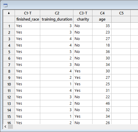In the final column, , we entered the name of the continuous independent variable, age, as follows: . The data setup is shown below:

Published with written permission from Minitab Inc.

Note: It does not matter which order you enter the variables into Minitab.

Minitab

Test Procedure in Minitab

In this section, we show you how to analyse your data using a binomial logistic regression in Minitab when the six assumptions set out in the Assumptions section have not been violated. Therefore, the six steps required to run a binomial logistic regression in Minitab are shown below:

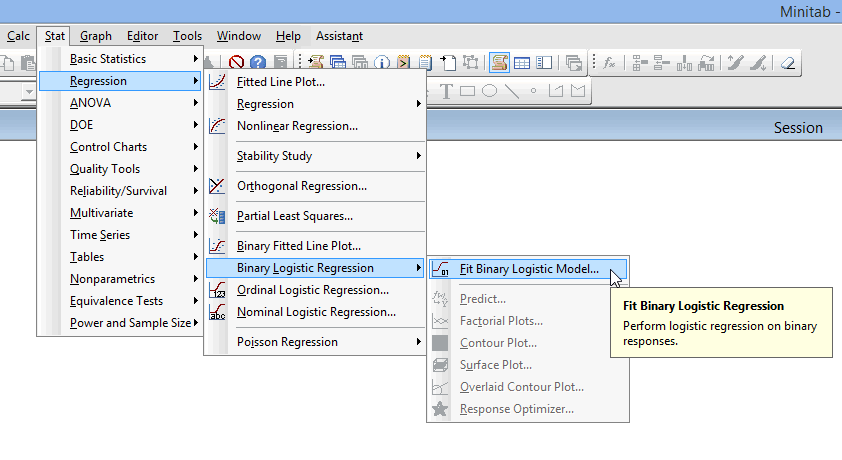
1. Click Stat > Regression > Binary Logistic Regression > Fit Binary Logistic Model... on the top menu, as shown below:
   

   Published with written permission from Minitab Inc.

   
   You will be presented with the following Binary Logistic Regression dialogue box
   
   

   Published with written permission from Minitab Inc.

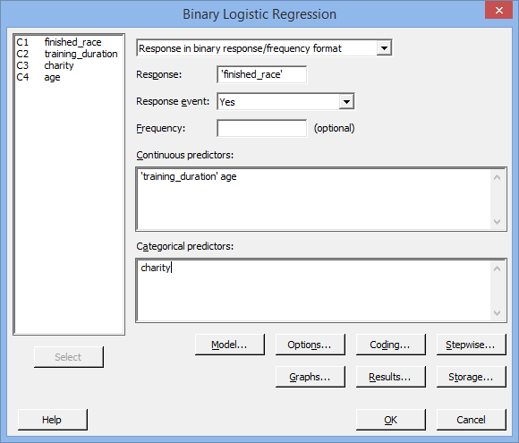
2. Transfer the dichotomous dependent variable, C1   finished_race, into the Response: box. Then, transfer the continuous independent variables – C2   training_duration and C4   age – into the Continuous predictors: box. Finally, transfer the categorical independent variable, C3   charity, into the Categorical predictors: box. You will end up with the following dialogue box:
   

   Published with written permission from Minitab Inc.

   Note: To transfer the various variables, you first need to click inside the various boxes (e.g., the Response: box) and all eligible variables that can be transferred will appear in the main left-hand box (e.g., C1   finished_race). This will activate the button (it is usually faded: ). Since the Response: box is where you put your dependent variable, you need to select the appropriate variable in the main left-hand box and either press the button or simply double-click on the variable (i.e., C1   finished_race in our example). You now need to follow the same procedure, but for the independent variables.

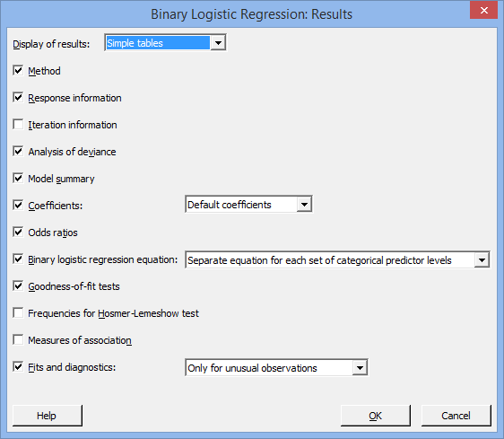
3. Click on the button. You will be presented with the Binary Logistic Regression: Results dialogue box, as shown below:
   

   Published with written permission from Minitab Inc.

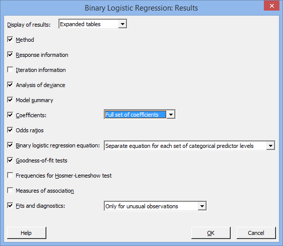
4. Change the Display of results: option to and the Coefficients: option to . You will be presented with the following:
   

   Published with written permission from Minitab Inc.

5. Click on the button. You will be returned to the Binary Logistic Regression dialogue box.
6. Click on the button. This will generate the results.

Minitab

Output of the binomial logistic regression in Minitab

You will notice that there is a lot of output produced by Minitab after you have run the binary logistic regression procedure. We summarize some of the most important parts of the output, as shown below:

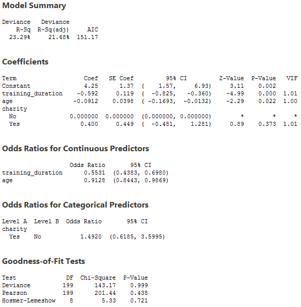
This output provides three important pieces of information:

• A. The Model Summary and Goodness-of-Fit Tests tables present statistics that try to assess how well the overall model (i.e., with all terms included in the model) fits the data. The Hosmer-Lemeshow test is one of the most popular methods and the result of this test is shown in the last row of the Goodness-of-Fit Tests table. Generally speaking, measures based on assessing the variability explained by the model are not well regarded methods of assessment of the model (e.g., the "Deviance R-Sq" column in the Model Summary table).
• B. The coefficients, as well as their statistical significance and other measures, are found in the Coefficients table. You can use this table to assess whether the terms in your model (e.g., age) are statistically significant (i.e., do they statistically significantly contribute to the model). For categorical independent variables, Minitab shows the dummy variables as well as the reference category used, so this is why you will always see one category with coefficients of 0.000000. You need to ignore this row. The value of the coefficients are found in the "Coef" column and the statistical significance of the coefficients are found in the "P-Value" column.
• C. The interpretation of the coefficients in their original form (as found in the Coefficients table) of a binomial logistic regression is unintuitive and, as such, Minitab provides the coefficients in odds ratio form, which are much more interpretable. The odds ratios for continuous independent variables and categorical independent variables are found in separate tables called the Odds Ratios for Continuous Predictors and Odds Ratios for Categorical Predictors tables, respectively. Odds ratios are often the values that are reported in research rather than the original coefficient values, although both can be reported.

In this example, the Hosmer-Lemeshow test is not statistically significant (p = .721), which indicates that the model fits the data well. The p-values for the training_duration, charity and age coefficients indicate that only training duration (p < .0005) and age (p = .022) are statistically significant predictors of dropout in a marathon race amongst first-time runners.

Note: A Classification Table is very useful to produce, but is not produced automatically by Minitab. Nonetheless, it can be produced in Minitab by selecting the correct options in the binary logistic regression procedure and following these up with further tests. Producing this table will allow you to calculate percentage accuracy in classification (PAC), Sensitivity, Specificity, positive predictive value and negative predictive value, all potentially useful measures in evaluating your data.

Minitab

Reporting the output of the binomial logistic regression

When you report the output of your binomial logistic regression, it is good practice to include:

• A. An introduction to the analysis you carried out.
• B. Information about your sample, including any missing values.
• C. An examination of all the assumptions of the binomial logistic regression, including any remedies that were taken for violations of any of these assumptions.
• D. A statement of how well the model fits the data using measures such as the Hosmer-Lemeshow test.
• E. The regression equation for your binomial logistic regression model, possibly including which coefficients/independent variables were statistically significant.
• F. The odds ratios reported for all coefficients/independent variables, including their statistical significance if not reported above.

Based on the Minitab output above, you could report the results as follows:

In addition to reporting the results as above, a diagram can be used to visually present your results. This can make it easier for others to understand your results. Furthermore, you can use Minitab to make predictions about dropout (the dependent variable) based on values you define for your independent variables. This is a separate procedure available in Minitab that you can use once you have run the binary logistic regression procedure.

Portions of information contained in this publication/book are printed with permission of Minitab Inc. All such material remains the exclusive property and copyright of Minitab Inc. All rights reserved.