Repeated Measures ANOVA (cont...)
Reporting the Result of a Repeated Measures ANOVA
We report the F-statistic from a repeated measures ANOVA as:
F(dftime, dferror) = F-value, p = p-value
which for our example would be:
F(2, 10) = 12.53, p = .002
This means we can reject the null hypothesis and accept the alternative hypothesis. As we will discuss later, there are assumptions and effect sizes we can calculate that can alter how we report the above result. However, we would otherwise report the above findings for this example exercise study as:
There was a statistically significant effect of time on exercise-induced fitness, F(2, 10) = 12.53, p = .002.
or
The six-month exercise-training programme had a statistically significant effect on fitness levels, F(2, 10) = 12.53, p = .002.
Tabular Presentation of a Repeated Measures ANOVA
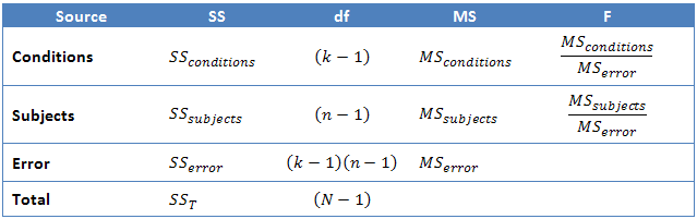
Normally, the result of a repeated measures ANOVA is presented in the written text, as above, and not in a tabular form when writing a report. However, most statistical programmes, such as SPSS Statistics, will report the result of a repeated measures ANOVA in tabular form. Doing so allows the user to gain a fuller understanding of all the calculations that were made by the programme. The table below represents the type of table that you will be presented with and what the different sections mean.
Most often, the Subjects row is not presented and sometimes the Total row is also omitted. The F-statistic found on the first row (time/conditions row) is the F-statistic that will determine whether there was a significant difference between at least two means or not. For our results, omitting the Subjects and Total rows, we have:
which is similar to the output produced by SPSS.
Increased Power in a Repeated Measures ANOVA
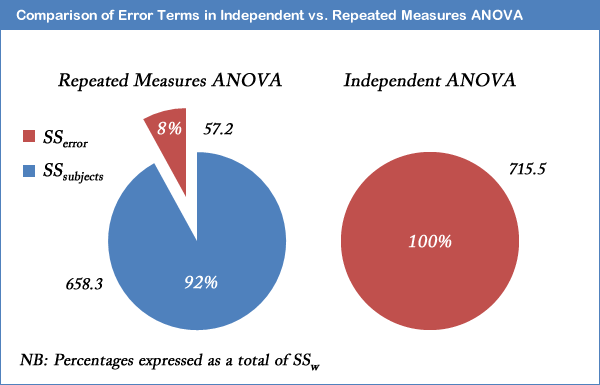
The major advantage with running a repeated measures ANOVA over an independent ANOVA is that the test is generally much more powerful. This particular advantage is achieved by the reduction in MSerror (the denominator of the F-statistic) that comes from the partitioning of variability due to differences between subjects (SSsubjects) from the original error term in an independent ANOVA (SSw): i.e. SSerror = SSw - SSsubjects. We achieved a result of F(2, 10) = 12.53, p = .002, for our example repeated measures ANOVA. How does this compare to if we had run an independent ANOVA instead? Well, if we ran through the calculations, we would have ended up with a result of F(2, 15) = 1.504, p = .254, for the independent ANOVA. We can clearly see the advantage of using the same subjects in a repeated measures ANOVA as opposed to different subjects. For our exercise-training example, the illustration below shows that after taking away SSsubjects from SSw we are left with an error term (SSerror) that is only 8% as large as the independent ANOVA error term.

This does not lead to an automatic increase in the F-statistic as there are a greater number of degrees of freedom for SSw than SSerror. However, it is usual for SSsubjects to account for such a large percentage of the within-groups variability that the reduction in the error term is large enough to more than compensate for the loss in the degrees of freedom (as used in selecting an F-distribution).
Effect Size for Repeated Measures ANOVA
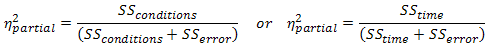
It is becoming more common to report effect sizes in journals and reports. Partial eta-squared is where the the SSsubjects has been removed from the denominator (and is what is produced by SPSS):
So, for our example, this would lead to a partial eta-squared of:
Underlying Assumptions: Normality
Similar to the other ANOVA tests, each level of the independent variable needs to be approximately normally distributed. How to check for this is provided in our Testing for Normality in SPSS Statistics guide.
Underlying Assumptions: Sphericity
The concept of sphericity, for all intents and purposes, is the repeated measures equivalent of homogeneity of variances. An explanation of sphericity is provided in our Sphericity guide. Testing for sphericity is an option in SPSS Statistics using Mauchly's Test for Sphericity as part of the GLM Repeated Measures procedure. Help with running a repeated measures ANOVA in SPSS Statistics can be found in our One-Way Repeated Measures ANOVA in SPSS Statistics guide. We can write up our results (not the exercise example), where we have included Mauchly's Test for Sphericity as:
Mauchly's Test of Sphericity indicated that the assumption of sphericity had been violated, χ2(2) = 22.115, p < .0005, and therefore, a Greenhouse-Geisser correction was used. There was a significant effect of time on cholesterol concentration, F(1.171, 38) = 21.032, p < .0005.